Abelianisation of logarithmic $$\mathfrak {sl}_2$$ -connections

Nikolaev, Nikita

doi:10.1007/s00029-021-00688-5

Abelianisation of logarithmic $\mathfrak {sl}_2$-connections

Open access
Published: 03 August 2021

Volume 27, article number 78, (2021)
Cite this article

Download PDF

You have full access to this open access article

Selecta Mathematica Aims and scope Submit manuscript

Abelianisation of logarithmic $\mathfrak {sl}_2$-connections

Download PDF

Nikita Nikolaev¹

1490 Accesses
4 Citations
4 Altmetric
Explore all metrics

Abstract

We prove a functorial correspondence between a category of logarithmic $\mathfrak {sl}_2$-connections on a curve ${\mathsf {X}}$ with fixed generic residues and a category of abelian logarithmic connections on an appropriate spectral double cover . The proof is by constructing a pair of inverse functors $\pi ^\text {ab}, \pi _\text {ab}$, and the key is the construction of a certain canonical cocycle valued in the automorphisms of the direct image functor $\pi _*$.

Lie groupoids and logarithmic connections

Article 04 April 2024

The locus of the representation of logarithmic connections by Fuchsian equations

Article Open access 30 March 2020

Differential characters and cohomology of the moduli of flat connections

Article 10 May 2018

Use our pre-submission checklist

Avoid common mistakes on your manuscript.

1 Introduction

This paper describes an approach to analysing meromorphic connections on Riemann surfaces. The technique, called abelianisation, is to introduce a decorated graph $\Gamma $ on a Riemann surface ${\mathsf {X}}$ in order to establish a correspondence between meromorphic connections on vector bundles of higher rank over ${\mathsf {X}}$ and meromorphic connections on line bundles (which we call abelian connections) over a multi-sheeted ramified cover . Namely, given a flat vector bundle ${{\mathcal {E}}}$ on ${\mathsf {X}}$, an application of the standard local theory of singular differential equations near each pole allows one to extract valuable asymptotic information in the form of locally defined flat filtrations on ${{\mathcal {E}}}$, first discovered by Levelt [18]. These filtrations, often called Levelt filtrations, can be organised into a single flat line bundle ${{\mathcal {L}}}$ over , and ${{\mathcal {E}}}$ can be recovered from ${{\mathcal {L}}}$ using the combinatorial data encoded in $\Gamma $.

1.1 Main result

In this paper, we restrict our attention to the simplest case of $\mathfrak {sl}_2$-connections with logarithmic singularities and generic residues. Our main result (Theorem 3.3) is a natural equivalence between a category of $\mathfrak {sl}_2$-connections on ${\mathsf {X}}$ and a category of logarithmic abelian connections on a double cover of ${\mathsf {X}}$. More precisely, fix $({\mathsf {X}},{\mathsf {D}})$ a compact smooth complex curve with a finite set of marked points, fix the data of generic residues along ${\mathsf {D}}$, and choose an appropriate meromorphic quadratic differential $\varphi $ on ${\mathsf {X}}$ with double poles along ${\mathsf {D}}$. Then $\varphi $ gives rise to a double cover (called the spectral curve) ramified at , a graph $\Gamma $ on ${\mathsf {X}}$ (called the Stokes graph), and a transversality condition on the Levelt filtrations extracted at nearby poles as dictated by $\Gamma $. Then there is a natural equivalence of categories:

Given a flat vector bundle ${{\mathcal {E}}}$ on ${\mathsf {X}}$, the abelianisation functor $\pi ^\text {ab}_\Gamma $ extracts Levelt filtrations along ${\mathsf {D}}$ and glues them into a flat line bundle ${{\mathcal {L}}}$ over . In order to recover ${{\mathcal {E}}}$ from ${{\mathcal {L}}}$, the main difficulty is that the naive guess that ${{\mathcal {E}}}$ is the pushforward $\pi _*{{\mathcal {L}}}$ is incorrect because $\pi _*{{\mathcal {L}}}$ necessarily has logarithmic singularities along the branch locus. The solution is to realise the combinatorial content of the Stokes graph $\Gamma $ in cohomology: we construct a canonical cocycle $\mathbb {V}$ on ${\mathsf {X}}$ (called the Voros cocycle) which deforms the pushforward functor $\pi _*$, as a functor, and this deformation is the nonabelianisation functor $\pi _\text {ab}^\Gamma $. The Voros cocycle is constructed in a completely standardised and combinatorial way from the Stokes graph $\Gamma $. This is significant because it means $\mathbb {V}$ is constructed without reference to any specific choice of ${{\mathcal {E}}}$ or ${{\mathcal {L}}}$, thereby setting up an equivalence of categories.

1.2 Context: spectral networks and exact WKB

Analysis of higher rank connections using abelian connections over a multi-sheeted cover has previously appeared in the context of spectral networks [7,8,9,10, 14], and even earlier from a different point of view in the context of the exact WKB analysis; e.g., [4, 16, 21]. The purpose of our work is to give a mathematical formulation of abelianisation of connections, and this paper is the first and important step in this direction. Our point of view, via the deformation theory of the pushforward functor, sheds light on the mathematical content of the methods of spectral networks and the exact WKB analysis, unifying the insights coming from these theories. Indeed, the local expressions for the Voros cocycle $\mathbb {V}$ involve precisely the same type of unipotent matrices that appear in the pioneering work of Voros on the exact WKB analysis [21] (we call $\mathbb {V}$ the Voros cocycle exactly for this reason). At the same time, the off-diagonal terms of $\mathbb {V}$ are given in terms of abelian parallel transports along canonically defined paths on the spectral curve. These appeared in the work of Gaiotto–Moore–Neitzke [8] which inspired the current project. In fact, one of the main achievements of this paper is giving a clear mathematical explanation that the path-lifting rule appearing in [8] emerges simply from the repeated application of the Voros cocycle.

1.3 Outlook

Abelianisation of connections can be seen as generalising the abelianisation of Higgs bundles [1, 13] (a.k.a. the spectral correspondence, which is a key step in the analysis of Hitchin integrable systems and the geometric Langlands programme) to flat bundles. Indeed, Proposition 3.6 shows that the abelianisation line bundle ${{\mathcal {L}}}$ is the correct analogue of the spectral line bundle. It was also conjectured in the work of Gaiotto–Moore–Neitzke [8] that such a procedure of abelianisation of connections should yield symplectic cluster coordinates on moduli spaces of meromorphic connections. This article (which is an extension of the work the author completed in his thesis [19]) is thus the first important step in realising this programme in mathematical terms.

1.4 Content

The article is dedicated to the proof of Theorem 3.3, which proceeds by constructing the functors $\pi ^\text {ab}_\Gamma , \pi _\text {ab}^\Gamma $ and showing that they form an inverse equivalence. Propositions 3.5 and 3.6 give a summary of the main properties of the relationship between $({{\mathcal {E}}}, \nabla )$ and its abelianisation . We also make the curious observation that the nonabelian Voros cocycle may itself be abelianised: there is an abelian cocycle on the spectral curve which completely determines the Voros cocycle $\mathbb {V}$ in the sense of Proposition 3.16.

2 Logarithmic connections and spectral curves

Throughout this paper, let ${\mathsf {X}}$ be a compact smooth complex curve and ${\mathsf {D}} \subset {\mathsf {X}}$ a finite set of marked points. We assume that ${\mathsf {D}}$ is nonempty with $|{\mathsf {D}}| > \chi ({\mathsf {X}}) = 2 - 2g_{\mathsf {X}}$, where $g_{\mathsf {X}}$ is the genus of ${\mathsf {X}}$. The Lie algebra $\mathfrak {sl} (2, \mathbb {C})$ is denoted by $\mathfrak {sl}_2$.

2.1 Logarithmic connections and Levelt filtrations

2.1. A logarithmic $\mathfrak {sl}_2$- connection on $({\mathsf {X}}, {\mathsf {D}})$ is the data $({{\mathcal {E}}}, \nabla , M )$ of a holomorphic rank-two vector bundle ${{\mathcal {E}}}$ on ${\mathsf {X}}$, a ${\underline{\mathbb {C}}}_{\mathsf {X}}$-linear map of sheaves

$$\begin{aligned} \nabla : {{\mathcal {E}}} \longrightarrow {{\mathcal {E}}} \otimes \Omega ^1_{\mathsf {X}} ({\mathsf {D}}) \end{aligned}$$

satisfying the Leibniz rule for all $e \in {{\mathcal {E}}}, f \in {{\mathcal {O}}}_{\mathsf {X}}$, and a trivialisation such that . They form a category, which we denote by $Conn ^2_{\mathfrak {sl}} ({\mathsf {X}},{\mathsf {D}})$. We will often omit “$ M $” from the notation.

2.2. Generic Levelt exponents and residue data. The residue sequence for $\Omega ^1_{\mathsf {X}} ({\mathsf {D}})$ implies that the restriction of $\nabla $ to ${\mathsf {D}}$ is a well-defined ${{\mathcal {O}}}_{\mathsf {D}}$-linear endomorphism , called the residue of $\nabla $ along ${\mathsf {D}}$. A further restriction of ${\text {Res}}\nabla $ to any point $\mathsf {p}\in {\mathsf {D}}$ is an endomorphism of the fibre whose eigenvalues $\pm \lambda _\mathsf {p}\in \mathbb {C}$ are called the Levelt exponents of $\nabla $ at $\mathsf {p}$. The determinant map sends ${\text {Res}}\nabla $ to a global section of ${{\mathcal {O}}}_{\mathsf {D}}$:

2.3 Definition

(Generic residue data) The Levelt exponents $\pm \lambda _\mathsf {p}$ at $\mathsf {p}$ are called generic if ${\text {Re}}(\lambda _\mathsf {p}) \ne 0$ and $\lambda _\mathsf {p}\notin \tfrac{1}{2} {\mathbb {Z}}$. We will refer to any section $a \in {\mathsf {H}}^0_{\mathsf {X}} ({{\mathcal {O}}}_{\mathsf {D}})$ as residue data, and say it is generic if for each $\mathsf {p}\in {\mathsf {D}}$, the two square roots $\pm \lambda _\mathsf {p}$ of $a_\mathsf {p}$ define generic Levelt exponents.

2.4. Thus, a is generic if and only if each complex number $a_\mathsf {p}$ is not purely negative real or a quarter square $n^2/4$ for some $n \in {\mathbb {Z}}$. We will always order the generic Levelt exponents by their increasing real part: $- \lambda _\mathsf {p}\prec \lambda _\mathsf {p}$ if and only if ${\text {Re}}(\lambda _\mathsf {p}) > 0$. The assumption that ${\text {Re}}(\lambda _\mathsf {p}) \ne 0$ is necessary for the construction in this paper because we will use the ordering $\prec $, but the assumption that $\lambda _\mathsf {p}\notin \tfrac{1}{2} {\mathbb {Z}}$ (usually called non-resonance) can be removed without a great deal of difficulty; in this paper, however, we restrict ourselves to this simplest situation and generalisations will appear elsewhere.

2.5 Example

Perhaps the most familiar explicit example is the following. Take ${\mathsf {X}} \mathrel {\mathop :}=\mathbb {P}^1$, fix $d \geqslant 3$ distinct points ${\mathsf {D}} \mathrel {\mathop :}=\left\{ u_1, \ldots , u_{d} \right\} \subset \mathbb {P}^1$, and d constant matrices $ A _1, \ldots , A _d \in \mathfrak {sl}_2$ with $ A _1 + \cdots + A _d = 0$. We usually choose an affine coordinate z on $\mathbb {P}^1 =\mathrel {\mathop :}\mathbb {P}^1_z$ such that $u_d$ is the point at infinity. Then the trivial rank-two vector bundle ${{\mathcal {E}}} = {{\mathcal {O}}}_{\mathbb {P}^1} \oplus {{\mathcal {O}}}_{\mathbb {P}^1}$ is equipped with a logarithmic connection $\nabla $ defined with respect to the standard basis for ${{\mathcal {E}}}$ by the following formula in the affine coordinate charts z and $w = z^{-1}$:

(1)

Evidently, $\nabla $ has logarithmic singularities at each point $u_i$ with residue ${\text {Res}}_{u_i} \nabla = A _i$. The residue ${\text {Res}}\nabla $ along ${\mathsf {D}}$ is then simply the full collection of the chosen matrices $\left\{ A _1, \ldots , A _d \right\} $. The eigenvalues $\pm \lambda _i \in \mathbb {C}$ of each $ A _i$ are the Levelt exponents of $\nabla $, so the residue data of $\nabla $ is $a = \left\{ \lambda _1^2, \ldots , \lambda _d^2 \right\} $.

2.6. The central object of study in this paper is the category of logarithmic $\mathfrak {sl}_2$-connections on $({\mathsf {X}},{\mathsf {D}})$ with fixed generic residue data a, for which we shall use the following shorthand notation:

2.7. Local diagonal decomposition. Fix a point $\mathsf {p}\in {\mathsf {D}}$, and consider a connection germ $({{\mathcal {E}}}_\mathsf {p}, \nabla _\mathsf {p})$ at $\mathsf {p}$ with generic Levelt exponents $\pm \lambda _\mathsf {p}$ at $\mathsf {p}$, where ${\text {Re}}(\lambda ) > 0$. A coordinate trivialisation transforms $\nabla _\mathsf {p}$ to a logarithmic $\mathfrak {sl}_2$-differential system , where is some $\mathfrak {sl}_2$-matrix of holomorphic function germs. By [22, Theorems 5.1, 5.4], there exists a holomorphic ${\mathsf {SL}}_2$ gauge transformation which transforms the given differential system into the diagonal system which depends only on $\lambda _\mathsf {p}$ and z. This classical theorem about singular ordinary differential equations admits vast generalisations, but we do not need them here. Together with the fixed ordering on the Levelt exponents, it induces a graded decomposition of ${{\mathcal {E}}}_\mathsf {p}$ with respect to which $\nabla _\mathsf {p}$ is diagonal.

2.8 Proposition

(Local diagonal decomposition) Let $({{\mathcal {E}}}_\mathsf {p}, \nabla _\mathsf {p}, M _\mathsf {p})$ be the germ of a logarithmic $\mathfrak {sl}_2$-connection at $\mathsf {p}\in {\mathsf {D}}$ with generic Levelt exponents $\pm \lambda _\mathsf {p}$. Then there is a canonical ordered decomposition

where is a rank-one logarithmic connection germ at $\mathsf {p}$ with residue $\pm \lambda _\mathsf {p}$. Moreover, $ M $ induces a flat skew-symmetric isomorphism .

Here, “skew-symmetric” means that $ M _\mathsf {p}$ is multiplied by $-1$ under the switching map. The order on the Levelt exponents $- \lambda _\mathsf {p}\prec + \lambda _\mathsf {p}$ determines a $\nabla _\mathsf {p}$-invariant filtration ${{\mathcal {E}}}_\mathsf {p}^\bullet \mathrel {\mathop :}=\big ( \Lambda ^-_\mathsf {p}\subset {{\mathcal {E}}}_\mathsf {p}\big )$ on the vector bundle germ ${{\mathcal {E}}}_\mathsf {p}$, which we will refer to as the Levelt filtration in reference to the more general such concept studied by Levelt in his thesis [18].

We will refer to the $\nabla _\mathsf {p}$-invariant filtration ${{\mathcal {E}}}_\mathsf {p}^\bullet \mathrel {\mathop :}=\big ( \Lambda ^-_\mathsf {p}\subset {{\mathcal {E}}}_\mathsf {p}\big )$, given by the order on the Levelt exponents $- \lambda _\mathsf {p}\prec + \lambda _\mathsf {p}$, as the Levelt filtration on the vector bundle germ ${{\mathcal {E}}}_\mathsf {p}$. Clearly, any pair of logarithmic $\mathfrak {sl}_2$-connection germs $({{\mathcal {E}}}_\mathsf {p}, \nabla _\mathsf {p}), ({{\mathcal {E}}}'_\mathsf {p}, \nabla '_\mathsf {p})$ with the same generic Levelt exponents $\pm \lambda _\mathsf {p}$ at $\mathsf {p}$ are isomorphic and any such isomorphism is necessarily diagonal with respect to the diagonal decompositions. Any morphism $({{\mathcal {E}}}_\mathsf {p}, \nabla _\mathsf {p}) \rightarrow ({{\mathcal {E}}}'_\mathsf {p}, \nabla '_\mathsf {p})$ necessarily preserves the Levelt filtration.

2.9 Example

Continuing Example 2.5, assume that $\nabla $ has generic residue data, and restrict our attention to the disc germ of, say, the singularity $u_1$. There is an ${\mathsf {SL}}_2$ matrix $ G = G (z)$, holomorphic at $z = u_1$, such that

Then the line subbundles $\Lambda _{1}^-, \Lambda _1^+$ are generated by $e_- \mathrel {\mathop :}= G ^{-1} {\tiny \begin{bmatrix}1\\ 0\end{bmatrix}}$ and $e_+ \mathrel {\mathop :}= G ^{-1} {\tiny \begin{bmatrix}0\\ 1\end{bmatrix}}$.

2.2 Logarithmic connections and double covers

Logarithmic connections can be pulled back and pushed forward along ramified covers. In this section we describe these operations, restricting ourselves to the simplest case of double covers with simple ramification and which are trivial over the polar divisor ${\mathsf {D}}$. Thus, let ${\mathsf {C}} \mathrel {\mathop :}=\pi ^{-1} ({\mathsf {D}})$ and let be the ramification divisor. Here and everywhere, we assume that ${\mathsf {R}}$ has no higher multiplicity and that the branch locus ${\mathsf {B}} \mathrel {\mathop :}=\pi ({\mathsf {R}}) \subset {\mathsf {X}}$ is disjoint from ${\mathsf {D}}$. We denote by the canonical involution.

2.10. Odd abelian connections. Connections on line bundles are sometimes called abelian connections. The line bundle carries a canonical logarithmic connection , defined to be the connection for which the canonical map is flat. Explicitly, if z is a local coordinate on vanishing at $\mathsf {r}\in {\mathsf {R}}$, then the local section gives a trivialisation, in which is given by

2.11 Definition

(Odd abelian connection) An odd abelian logarithmic connection on is the data consisting of an abelian logarithmic connection on equipped with a skew-symmetric isomorphism intertwining and .

Here, “skew-symmetric” means $\mu $ satisfies $\sigma ^*\mu = - \mu $. Abelian connections with a similar structure but over the punctured curve have appeared in [14, §4.2] under the name equivariant connections. We refer to the isomorphism $\mu $ as the odd structure on . Odd abelian connections form a category

where morphisms are morphisms of connections $\phi : {{\mathcal {L}}} \rightarrow {{\mathcal {L}}}'$ that intertwine the odd structures $\mu , \mu '$ in the sense that $\mu ' \circ (\phi \otimes \sigma ^*\phi ) = \mu $. It is easy to check that if $\mu _1, \mu _2$ are any two odd structures on the same abelian connection , then , and there are exactly two such isomorphisms.

2.12 Proposition

(Residues of odd connections) The residue of any odd abelian connection at a ramification point is $-1/2$. In particular, the monodromy of around a ramification point is $-1$. Furthermore, if $\mathsf {p}\in {\mathsf {D}}$ and $\mathsf {p}_\pm \in {\mathsf {C}}$ are the two preimages of $\mathsf {p}$, then the residues of at $\mathsf {p}_\pm $ satisfy

Proof

The residue of at $\mathsf {r}\in {\mathsf {R}}$ is $-1$. If , then the residue of the connection at $\mathsf {r}$ is $2 \lambda $, so the odd structure on ${{\mathcal {L}}}$ forces $\lambda = -1/2$. Next, since $\sigma (\mathsf {p}_-) = \mathsf {p}_+$, the residue at $\mathsf {p}_-$ of is equal to the residue of at $\mathsf {p}_+$. This means has residue at $\mathsf {p}_-$. But the residue of at $\mathsf {p}_-$ is 0, so the odd structure on ${{\mathcal {L}}}$ forces the identity. $\square $

By using the residue theorem for connections [6, Cor. (B.3), p.186], it is easy to compute the degree of a line bundle carrying an odd connection.

2.13 Proposition

(Degree of odd connections) If , then .

2.14. Pullback and pushforward of connections. The pullback of ${{\mathcal {O}}}_{\mathsf {X}}$-modules along $\pi $ extends to a pullback functor on connections

by the rule $\pi ^*\nabla (\pi ^*e) = \pi ^*(\nabla e)$ for any local section $e \in {{\mathcal {E}}}$. Clearly, the Levelt exponents of $\nabla $ at $\mathsf {p}\in {\mathsf {D}}$ and the Levelt exponents of $\pi ^*\nabla $ at any preimage $\tilde{\mathsf {p}} \in {\mathsf {C}}$ of $\mathsf {p}$ are the same. More interesting is pushing connections forward along $\pi $. The direct image functor $\pi _*$ of -modules can be used to pushforward connections from down to ${\mathsf {X}}$, but the relationship between the polar divisors is more complicated (see [11, proposition 2.17] for more generality).

2.15 Proposition

(Pushforward of odd abelian connections) The direct image $\pi _*$ extends to a functor

(2)

Moreover, for any , if $\pm \lambda \in \mathbb {C}$ are its residues at the two preimages $\mathsf {p}_\pm \in {\mathsf {C}}$ of a point $\mathsf {p}\in {\mathsf {D}}$, then the Levelt exponents of at $\mathsf {p}$ are $\pm \lambda $.

Proof

A logarithmic connection on is a map , and its direct image is therefore . We claim that there is a canonical isomorphism . First, $\pi ^*\Omega ^1_{\mathsf {X}} ({\mathsf {B}} \cup {\mathsf {D}}) = \big ( \pi ^*\Omega ^1_{\mathsf {X}} \big ) ( \pi ^*({\mathsf {B}} \cup {\mathsf {D}}))$, where $\pi ^*({\mathsf {B}} \cup {\mathsf {D}}) = 2{\mathsf {R}} \cup {\mathsf {C}}$ (pulled back as a divisor). The derivative map drops rank along ${\mathsf {R}}$; i.e., it is a nonvanishing section of the line bundle , thereby inducing an isomorphism . Dualising, we get . Thus, the projection formula implies . To check that satisfies the Leibniz rule, let $e \in \pi _*{{\mathcal {L}}}$ be a local section on some open set ${\mathsf {U}} \subset {\mathsf {X}}$, and $f \in {{\mathcal {O}}}_{\mathsf {X}} ({\mathsf {U}})$. Then . Now it is clear that the Leibniz rule for follows from the Leibniz rule for . Therefore, is a rank-two logarithmic connection on $({\mathsf {X}}, {\mathsf {B}} \cup {\mathsf {D}})$.

To show that the odd structure on ${{\mathcal {L}}}$ induces an $\mathfrak {sl}_2$-structure on $\pi _*{{\mathcal {L}}}$, recall that there is a canonical isomorphism , where ${\text {Nm}}({{\mathcal {L}}})$ is the norm of ${{\mathcal {L}}}$ [12, Cor. 3.12]. For a double cover, there is a canonical isomorphism $\pi ^*{\text {Nm}}({{\mathcal {L}}}) \cong {{\mathcal {L}}} \otimes \sigma ^*{{\mathcal {L}}}$. Moreover, it is easy to see that is canonically isomorphic to . The statement about the residues is obvious because $\pi $ is unramified over ${\mathsf {D}}$. $\square $

2.16. Image of $\pi _*$. One can show that the monodromy of around the branch locus ${\mathsf {B}}$ is a quasi-permutation representation of the double cover [17]. As a result, no connection on $({\mathsf {X}},{\mathsf {D}})$ is the pushforward of an abelian connection on . In other words, the image of the pushforward functor $\pi _*$ in $Conn ^2_{\mathfrak {sl}} ({\mathsf {X}}, {\mathsf {B}} \cup {\mathsf {D}})$ does not even intersect the subcategory $Conn ^2_{\mathfrak {sl}} ({\mathsf {X}}, {\mathsf {D}})$. Abelianisation fixes this problem: in Sect. 3.3, we will explicitly construct a deformation of the pushforward functor $\pi _*$ which does map into $Conn ^2_{\mathfrak {sl}} ({\mathsf {X}}, {\mathsf {D}})$.

2.3 Spectral curves for quadratic differentials

Let $\varphi $ be a quadratic differential on $({\mathsf {X}},{\mathsf {D}})$, by which we mean a meromorphic quadratic differential on ${\mathsf {X}}$ with at most order-two poles along ${\mathsf {D}}$; i.e., it is a global holomorphic section of ${\mathsf {S}}^2 \Omega ^1_{\mathsf {X}} (2{\mathsf {D}})$. The standard reference is [20]; see also [3, §§2,3]. By the Riemann–Roch Theorem,

(3)

2.17. Quadratic residue. In any local coordinate x centred at $\mathsf {p}\in {\mathsf {D}}$, a quadratic differential $\varphi $ with a double pole at $\mathsf {p}$ is expanded as . The coefficient $a_\mathsf {p}\in \mathbb {C}$ is a coordinate-independent quantity, called the (quadratic) residue of $\varphi $ at $\mathsf {p}$ and denoted ${\text {Res}}_\mathsf {p}(\varphi )$. The residue of $\varphi $ along ${\mathsf {D}}$ is thus a global section $a = {\text {Res}}(\varphi ) \in {\mathsf {H}}^0_{\mathsf {X}} ({{\mathcal {O}}}_{\mathsf {D}})$, same as what we called residue data in Sect. 2.1. There is a quadratic residue short exact sequence:

(4)

2.18 Lemma

For any $a \in {\mathsf {H}}^0_{\mathsf {X}} ({{\mathcal {O}}}_{\mathsf {D}})$, there is a quadratic differential $\varphi $ on $({\mathsf {X}},{\mathsf {D}})$ with ${\text {Res}}(\varphi ) = a$.

Proof

By the Kodaira Vanishing Theorem, ${\mathsf {H}}^1_{\mathsf {X}} \big ( {\mathsf {S}}^2 \Omega ^1_{\mathsf {X}} ({\mathsf {D}}) \big ) = 0$, which implies that the residue map ${\text {Res}}: {\mathsf {H}}^0_{\mathsf {X}} \big ( {\mathsf {S}}^2 \Omega ^1_{\mathsf {X}} (2{\mathsf {D}}) \big ) \rightarrow {\mathsf {H}}^0_{\mathsf {X}} \big ( {{\mathcal {O}}}_{\mathsf {D}} \big )$ is surjective. This means that any residue data a decorating the divisor ${\mathsf {D}}$ can be lifted to a quadratic differential $\varphi $. $\square $

2.19. In view of (3), the only configuration $({\mathsf {X}},{\mathsf {D}})$ for which there is a unique quadratic differential $\varphi $ with specified residues is $(g_{\mathsf {X}}, |{\mathsf {D}}|) = (0,3)$ (i.e., $\mathbb {P}^1$ with three marked points). In this case, the three-dimensional vector space of quadratic differentials ${\mathsf {H}}^0_{\mathsf {X}} \big ( {\mathsf {S}}^2 \Omega ^1_{\mathsf {X}} (2{\mathsf {D}}) \big )$ can be parameterised by the residues $\alpha , \beta , \gamma $ at the three points of ${\mathsf {D}}$. Identifying $({\mathsf {X}}, {\mathsf {D}})$ with $(\mathbb {P}^1, \left\{ 0,1,\infty \right\} )$, one can show that the unique quadratic differential with residues $\alpha , \beta , \gamma $ at the double poles $0,1, \infty $ is

(5)

2.20. Generic quadratic differentials. We will say that a quadratic differential $\varphi $ is generic if all zeroes are simple. The subspace of generic quadratic differentials in ${\mathsf {H}}^0_{\mathsf {X}} \big ( {\mathsf {S}}^2 \Omega ^1_{\mathsf {X}} (2{\mathsf {D}}) \big )$ is obviously open dense given as the complement of a hypersurface. If $(g_{\mathsf {X}}, |{\mathsf {D}}|) \ne (0,3)$, then the space of quadratic differentials is at least one-dimensional; but if $(g_{\mathsf {X}}, |{\mathsf {D}}|) = (0,3)$, this is a condition on the residues of $\varphi $. One can use (5) to calculate that the open subspace of generic quadratic differentials for $(g_{\mathsf {X}}, |{\mathsf {D}}|) = (0,3)$ is the complement of the quadratic hypersurface

(6)

2.21 Lemma

Let $a \in {\mathsf {H}}^0_{\mathsf {X}} ({{\mathcal {O}}}_{\mathsf {D}})$ be generic residue data. If $(g_{\mathsf {X}}, |{\mathsf {D}}|) = (0, 3)$, assume in addition that a is contained in the complement of the hypersurface (6). Then there exists a generic quadratic differential $\varphi $ on $({\mathsf {X}},{\mathsf {D}})$ such that ${\text {Res}}(\varphi ) = a$.

2.22 Example

Consider the following examples of meromorphic quadratic differentials on ${\mathsf {X}} \mathrel {\mathop :}=\mathbb {P}^1_z$:

The quadratic differential $\varphi _1$ is of the form (6) with $\alpha = \beta = \gamma = 1/9$. They respectively have double poles along ${\mathsf {D}}_1 \mathrel {\mathop :}=\left\{ 0, 1, \infty \right\} $, ${\mathsf {D}}_2 \mathrel {\mathop :}=\left\{ 0, \pm 1, \infty \right\} $, and ${\mathsf {D}}_3 \mathrel {\mathop :}=\left\{ e^{\pm \pi i /4}, e^{\pm 3\pi i /4} \right\} $. Each quadratic residue of $\varphi _1$ and $\varphi _2$ is 1/9; each quadratic residue of $\varphi _3$ is $e^{\pi i /4}$. The quadratic differential $\varphi _1$ has two simple zeros at $e^{\pm \pi i/3}$. The quadratic differentials $\varphi _2, \varphi _3$ both have four simple zeros; they are respectively $e^{\pm \pi i/4}, e^{\pm 3\pi i/4}$ and $\pm \tfrac{1}{2} e^{\pi i/4}, \pm 2 e^{3\pi i/4}$. Consequently, all three of these quadratic differentials are generic with generic residues.

2.23. The log-cotangent bundle. Let ${\mathsf {Y}}$ be the total space of $\Omega ^1_{\mathsf {X}} ({\mathsf {D}})$, sometimes called the log-cotangent bundle, and let $p : {\mathsf {Y}} \rightarrow {\mathsf {X}}$ be the projection map. Like the usual cotangent bundle, the log-cotangent bundle ${\mathsf {Y}}$ has a canonical one-form, which can be constructed as follows. Let $\theta \in {\mathsf {H}}^0 \big ({\mathsf {Y}}, p^*\Omega ^1_{\mathsf {X}} ({\mathsf {D}}) \big )$ be the tautological section. Then the fibre product

exists in the category of vector bundles, because $p : {\mathsf {Y}} \rightarrow {\mathsf {X}}$ is a surjective submersion. Unravelling the definition of the fibre product, we find that ${{\mathcal {A}}}$ consists of all vector fields on ${\mathsf {Y}}$ that are tangent to the divisor $p^*{\mathsf {D}} \subset {\mathsf {Y}}$; i.e., ${{\mathcal {A}}} \cong {{\mathcal {T}}}_{\mathsf {Y}} (- \log p^*{\mathsf {D}})$. Finally, dualising the surjective map ${{\mathcal {A}}} \rightarrow p^*{{\mathcal {T}}}_{\mathsf {X}} (-{\mathsf {D}})$ yields an injective morphism . The canonical one-form $\eta _{\mathsf {Y}} \in {\mathsf {H}}^0 \big ( {\mathsf {Y}}, \Omega ^1_{\mathsf {Y}} (\log p^*{\mathsf {D}}) \big )$ on ${\mathsf {Y}}$ is then defined as the image of the tautological section $\theta $ under this map.

2.24 Example

Take ${\mathsf {X}} = \mathbb {P}^1_z$ with ${\mathsf {D}} = \left\{ 0,1,\infty \right\} $. Then $\Omega ^1_{\mathbb {P}^1} ({\mathsf {D}})$ has a trivialisation over the affine z-chart given by the logarithmic one-form . With respect to this trivialisation, the canonical one-form $\eta _ Y $ is simply where y is the linear coordinate in the fibre.

2.25. The spectral curve. If $\varphi $ is a quadratic differential on $({\mathsf {X}},{\mathsf {D}})$, then $p^*\varphi $ is a section of ${\mathsf {S}}^2 \big ( \Omega ^1_{\mathsf {Y}} (\log p^*{\mathsf {D}}) \big )$ via . The spectral curve of $\varphi $ is the zero locus in ${\mathsf {Y}}$ of the section $\eta ^2_{\mathsf {Y}} - p^*\varphi \in {\mathsf {S}}^2 \big ( \Omega ^1_{\mathsf {Y}} (\log p^*{\mathsf {D}}) \big )$:

(7)

We denote by the restriction to of the canonical projection $p : {\mathsf {Y}} \rightarrow {\mathsf {X}}$. We also denote the ramification divisor by and the branch divisor by ${\mathsf {B}} \subset {\mathsf {X}}$. As a double cover, is equipped with a canonical involution .

If $\varphi $ is generic, then is embedded in ${\mathsf {Y}}$ as a smooth divisor, and the projection is a simply ramified double cover, branched exactly at the zeroes of $\varphi $, and trivial over the points of ${\mathsf {D}}$. Its genus is . (see, e.g., [1, remark 3.2]). Using the Riemann–Hurwitz formula, the number of ramification points $|{\mathsf {R}}|$ of $\pi $, which is the same as the number of zeroes $|{\mathsf {B}}|$ of $\varphi $, is

(8)

2.26 Example

For the quadratic differential $\varphi _1$ from Example 2.22, the spectral curve has genus 0, hence is a copy of $\mathbb {P}^1$. If we trivialise $\Omega ^1_{\mathbb {P}^1} ({\mathsf {D}})$ over the affine z-chart using the differential form , then is given by the equation $y^2 = \tfrac{1}{9} (z^2 - z + 1)$. For both quadratic differentials $\varphi _2$ and $\varphi _3$, the spectral curve has genus 1, so it is an elliptic curve over $\mathbb {P}^1$, and it is given by $y^2 = \tfrac{1}{9} (z^4 + 1)$.

Notice that, although the quadratic differential $\varphi _1$ is singular at the points 0, 1 in the affine z-chart, its spectral curve is perfectly well-behaved above these points (see Fig. 1). This is a manifestation of the fact that our spectral curve is embedded inside the total space of the logarithmic cotangent bundle rather than the usual cotangent bundle. In contrast, constructing a spectral curve of $\varphi _1$ using the same equations but in the usual cotangent bundle yields a curve which escapes from the total space above the points 0, 1 (see Fig. 2).

2.27. The canonical one-form. Pulling back the canonical one-form $\eta _{\mathsf {Y}}$ to yields a differential form $\eta $ with logarithmic poles along ${\mathsf {C}} \mathrel {\mathop :}=\pi ^{-1} ({\mathsf {D}})$, called the canonical one-form on . It satisfies $\eta ^2 = \pi ^*\varphi $ and $\sigma ^*\eta = - \eta $, and can therefore be thought of as the ‘canonical square root’ of the quadratic differential $\varphi $. It has zeroes along the ramification locus ${\mathsf {R}}$, and its residues at the two preimages $\mathsf {p}_\pm \in {\mathsf {C}}$ of any point $\mathsf {p}\in {\mathsf {D}}$ satisfy ${\text {Res}}_{\mathsf {p}_-} \eta = - {\text {Res}}_{\mathsf {p}_+} \eta $ and $\big ( {\text {Res}}_{\mathsf {p}_\pm } \eta \big )^2 = {\text {Res}}_\mathsf {p}\varphi $. If the residue data $a = {\text {Res}}(\varphi )$ is generic, we can fix an order on the preimages of $\mathsf {p}$:

(9)

If $\mathsf {p}_- \prec \mathsf {p}_+$, we shall call $\mathsf {p}_-$ a sink pole and $\mathsf {p}_+$ a source pole. The divisor ${\mathsf {C}}$ is thus decomposed equally into sinks and sources ${\mathsf {C}} = {\mathsf {C}}^- \sqcup {\mathsf {C}}^+$.

2.4 Logarithmic connections and spectral curves

In general, connections do not have an invariant notion of eigenvalues or eigenvectors. However, in the presence of a spectral curve, we can make sense of these notions as follows.

2.28.

Let be the spectral curve of a generic quadratic differential $\varphi $ with generic residue data a along ${\mathsf {D}}$. Suppose $({{\mathcal {E}}}, \nabla ) \in Conn _{\mathsf {X}}^2$ is a logarithmic $\mathfrak {sl}_2$-connection on $({\mathsf {X}},{\mathsf {D}})$ with residue data a. If $\mathsf {p}\in {\mathsf {D}}$, let $\pm \lambda _\mathsf {p}$ be the Levelt exponents at $\mathsf {p}$, which by construction are the residues of $\eta $ at the preimages $\mathsf {p}_\pm \in {\mathsf {C}}$. Consider the local diagonal decomposition ${{\mathcal {E}}}_\mathsf {p}\cong \Lambda _\mathsf {p}^- \oplus \Lambda _\mathsf {p}^+$.

Let z be a local coordinate on centred at $\mathsf {p}_\pm $ in which $\eta $ is in normal form . Since is unramified over $\mathsf {p}$, we also use z as a local coordinate on ${\mathsf {X}}$ centred at $\mathsf {p}$. If we fix a basepoint $\mathsf {p}_*$ near $\mathsf {p}$, then examining the Levelt normal form of $\nabla _\mathsf {p}$ with respect to the coordinate z we obtain germs of (multivalued) flat sections $\psi ^\pm _\mathsf {p}$ which can be expressed as $\psi ^\pm _\mathsf {p}= f^\pm _\mathsf {p}e^\pm _\mathsf {p}$, where $e^\pm _\mathsf {p}$ is a (univalued) generator of $\Lambda _\mathsf {p}^\pm $, and $f^\pm _\mathsf {p}$ is the germ of a (multivalued) function defined in the coordinate z by The observation is that the integrand in this expression is precisely the canonical one-form $\eta $ thought of as written in the local coordinate z near $\mathsf {p}$.

2.29.

To express this in a coordinate-free way, let ${\mathsf {U}} \subset {\mathsf {X}}$ be any simply connected open neighbourhood of $\mathsf {p}$ disjoint from ${\mathsf {B}}$ and all other points of ${\mathsf {D}}$. Then ${\mathsf {U}}$ has two disjoint preimages ${\mathsf {U}}_\pm $ on where ${\mathsf {U}}_\pm $ contains $\mathsf {p}_\pm $. Let $\eta _\pm $ be the restriction of $\eta $ to ${\mathsf {U}}_\pm $, and we can think of $\eta _\pm $ as being defined on ${\mathsf {U}}$. Define (multivalued) functions on the punctured neighbourhood ${\mathsf {U}}^\circ \mathrel {\mathop :}={\mathsf {U}} \setminus \left\{ \mathsf {p} \right\} $ by $ f_\pm (\mathsf {q}) \mathrel {\mathop :}=\exp \left( - \int _{\mathsf {p}_*}^\mathsf {q}\eta _\pm \right) . $ Note that the germ of $f_\pm $ at $\mathsf {p}$ is precisely $f_\mathsf {p}^\pm $, and that $f_\pm $ satisfies the differential equation ; moreover, $f_\pm $ is nowhere-vanishing on ${\mathsf {U}}^\circ $. Analytically continue the solutions $\psi ^\pm _\mathsf {p}$ to multivalued flat sections $\psi _\pm $ of ${{\mathcal {E}}}$ over ${\mathsf {U}}^\circ $, and define $ e_\pm \mathrel {\mathop :}=f_\pm ^{-1} \psi _\pm . $ These sections of ${{\mathcal {E}}}$ form a basis of holomorphic generators over ${\mathsf {U}}$ satisfying:

Thus, we can think of $e_\pm $ as an eigensection of $\nabla $ with eigenvalue $\eta _\pm $, and the line subbundles that they generate determine the flat eigen-decomposition of $({{\mathcal {E}}}, \nabla )$ over ${\mathsf {U}}$ that uniquely continues the local diagonal decomposition of ${{\mathcal {E}}}_\mathsf {p}$:

2.30.

More invariantly, let be any simply connected neighbourhood of a pole which is disjoint from ${\mathsf {R}}$ and all other points of ${\mathsf {C}}$. Let f be any (multivalued) solution of the differential equation defined over the punctured neighbourhood $\tilde{{\mathsf {U}}}^*\mathrel {\mathop :}=\tilde{{\mathsf {U}}} \setminus \left\{ \mathsf {p} \right\} $. Then the same calculation as above shows that the pullback $\pi ^*{{\mathcal {E}}}$ over $\tilde{{\mathsf {U}}}$ has a section e which is an eigensection of $\pi ^*\nabla $ with eigenvalue $\eta $:

2.5 The Stokes graph

Fix some generic residue data a. If $(g_{\mathsf {X}}, |{\mathsf {D}}|) = (0, 3)$, assume in addition that a is contained in the complement of the hypersurface (6). For any generic quadratic differential $\varphi $ on $({\mathsf {X}},{\mathsf {D}})$ with residues a, let be its spectral curve with canonical one-form $\eta $.

2.31. The horizontal foliation. The curves ${\mathsf {X}}$ and , viewed as real two-dimensional surfaces, are naturally equipped with singular foliations $\mathfrak {F}$ and , respectively, with the property that is the orientation double cover of $\mathfrak {F}$. These foliations are well-known (see, e.g., [15, 20]), and we only recall what is necessary (see [3, §3] for a concise survey). The foliation can be defined as the integration of the real distribution ${ker} \big ( {\text {Im}}(\eta ) \big )$ inside the real tangent bundle of . Concretely, the local equation for a leaf passing through a point $\mathsf {p}$ is given by ${\text {Im}}\left( \, \int _{\mathsf {p}}^{\mathsf {z}} \eta \, \right) = 0$. Evidently, this foliation is singular at the poles ${\mathsf {C}} = \pi ^{-1} ({\mathsf {D}})$ and at the ramification points ${\mathsf {R}}$. The foliation $\mathfrak {F}$, defined as the image of under $\pi $, is often called the horizontal foliation for the quadratic differential $\varphi $; it is singular at the poles ${\mathsf {D}}$ and the branch points ${\mathsf {B}}$. A leaf of $\mathfrak {F}$ (or ) is critical if one of its endpoints belongs to ${\mathsf {B}}$ (or ${\mathsf {R}}$). A critical leaf of $\mathfrak {F}$ is a saddle trajectory if both of its endpoints belong to ${\mathsf {B}}$.

2.32.

If the horizontal foliation $\mathfrak {F}$ has no saddle trajectories, then by [3, Lemma 3.1] the open real surface ${\mathsf {X}} \setminus ({\mathsf {D}} \cup {\mathsf {B}} \cup \Gamma )$, where $\Gamma $ is the union of all critical leaves of $\mathfrak {F}$, decomposes into a finite disjoint union of topological open discs, called horizontal strips (Fig. 3). Similarly, the open real surface , where is the union of all critical leaves of , is also a finite disjoint union of horizontal strips (Fig. 3).

2.33. Saddle-free quadratic differentials and very generic residues. If the horizontal foliation $\mathfrak {F}$ has no saddle trajectories, then the quadratic differential $\varphi $ is said to be saddle-free. It follows from [3, Lemma 4.11] that the subset of quadratic differentials which are saddle-free is open dense. Note that “saddle-free” may be a condition on the residue data a. For example, if $(g_{\mathsf {X}}, |{\mathsf {D}}|) = (0, 3)$, the quadratic differential $\varphi $ with given residues a is unique (given by (5)) and may fail to be saddle-free. In this case, there are only two ramification points , so a saddle trajectory occurs if and only if the canonical one-form $\eta $ satisfies ${\text {Im}}\left( \, \int _{\mathsf {r}_-}^{\mathsf {r}_+} \eta \, \right) = 0$ for a path of integration in . If $\mathsf {b}_\pm \in {\mathsf {B}}$ are the two branch points, then upon identifying ${\mathsf {X}} \cong \mathbb {P}^1$ and choosing a branch cut in order to write $\eta $ with $\sqrt{\varphi }$, where $\varphi $ is given by (5), this integral can be explicitly computed in terms of logarithms and it defines a closed real-analytic subset of $\mathbb {C}^3_{\alpha \beta \gamma }$. It therefore determines an explicit condition on the residues $a = \left\{ \alpha , \beta , \gamma \right\} $ for the unique $\varphi $ to be saddle-free. We will say that residue data a is very generic if there exists a generic saddle-free quadratic differential $\varphi $ with residues a.

Ultimately, however, this apparent rigidity in our construction is artificial and can be removed by using a more topological argument. We will study this as well as other non-generic situations elsewhere.

2.34 Example

All three quadratic differentials $\varphi _1, \varphi _2, \varphi _3$ from Example 2.22 are saddle-free. The true plots of their critical trajectories are presented in Fig. 4.

2.35. The Stokes and spectral graphs Now we define the main combinatorial gadgets in our construction. Let $\varphi $ be a generic and saddle-free quadratic differential.

2.36 Definition

(Stokes graph, spectral graph) The Stokes graph $\Gamma $ is the graph on ${\mathsf {X}}$ whose vertices are ${\mathsf {D}} \cup {\mathsf {B}}$ and whose edges are the critical leaves of $\mathfrak {F}$. The spectral graph is the oriented graph on whose vertices are ${\mathsf {C}} \cup {\mathsf {R}}$ and whose edges are the critical leaves of .

Thus, is a (ramified) orientation double cover of graphs. Each face of $\Gamma $ and is a horizontal strip. We refer to the edges and the faces of $\Gamma $ as Stokes rays and Stokes regions; and to the edges and the faces of as spectral rays and spectral regions. The graphs are bipartite with bipartitions $\Gamma _0 = {\mathsf {D}} \cup {\mathsf {B}}$ and .

The polar vertices ${\mathsf {C}}$ are further divided into sinks and sources (cf. 2.27):

sink vertices $\mathrm{{\mathsf {C}}_-}$: those where ${\text {Re}}({\text {Res}}\eta ) < 0$;
source vertices $\mathrm{{\mathsf {C}}_+}$: those where ${\text {Re}}({\text {Res}}\eta ) > 0$.

If $\mathsf {p}\in {\mathsf {D}}$, we will always denote its preimages in ${\mathsf {C}}$ by $\mathsf {p}_-, \mathsf {p}_+$ where $\mathsf {p}_\pm \in {\mathsf {C}}_\pm $. They satisfy the relation $\sigma (\mathsf {p}_\pm ) = \mathsf {p}_\mp $. All spectral rays incident to a sink/source are oriented into/out of the sink/source, so spectral rays are divided by parity:

positive spectral rays : polar vertex is a source;
negative spectral rays : polar vertex is a sink.

2.37.

Spectral rays always occur in pairs: the involution $\sigma $ maps a spectral ray to a spectral ray of opposite parity. Stokes rays have no natural notion of parity; instead, the preimage of every Stokes ray $\alpha \in \Gamma _1$ is a pair of opposite spectral rays (see Fig. 5). The graphs are squaregraphs: every Stokes region is a quadrilateral with two branch vertices and two polar vertices, and its boundary is made up of four Stokes rays (Fig. 6).

Similarly, every spectral region is a quadrilateral with two ramification vertices and two polar vertices (one of which is a source and one is a sink), and its boundary is made up of four spectral rays (two of which are positive and two are negative). We index them as described in Fig. 6:

Each branch point has three incident Stokes rays and three incident Stokes regions, but each Stokes region has two branch vertices, so there are $3|{\mathsf {B}}|$ Stokes rays and $\tfrac{3}{2}|{\mathsf {B}}|$ Stokes regions in total. So, using (8),

(10)

(11)

Note also that .

2.38 Example

Figure 4 shows a plot of the Stokes graph of the quadratic differential $\varphi _1$ from Example 2.22. Figure 7 shows a more schematic rendering.

2.39. The Stokes open cover. The graphs define canonical acyclic open covers (i.e., every finite intersection is either empty or a disjoint union of contractible open sets) of the punctured curves

by enlarging all edges and faces as follows. For every face $ I \in \Gamma _2$ and every edge $\alpha \in \Gamma _1$, let ${\mathsf {U}}_{ I }$ and ${\mathsf {U}}_{\alpha }$ be the germs of open neighbourhoods in ${\mathsf {X}}^\circ $ of the face $ I $ and the edge $\alpha $, respectively. We continue calling them Stokes regions and Stokes rays. We define spectral regions ${\mathsf {U}}_i$ and spectral rays ${\mathsf {U}}_\alpha ^\pm $ for all in the same way. We obtain what we call Stokes open covers of ${\mathsf {X}}^\circ $ and , respectively:

(12)

If $\mathsf {p}$ is a vertex of ${\mathsf {U}}_ I $, then intersecting ${\mathsf {U}}_ I $ with the infinitesimal disc ${\mathsf {U}}_\mathsf {p}$ around $\mathsf {p}$ can be seen as the germ of a sectorial neighbourhood of $\mathsf {p}$ (or a disjoint union of two). In fact, the infinitesimal punctured disc ${\mathsf {U}}_\mathsf {p}^*$ centred at $\mathsf {p}$ is covered by such sectorial neighbourhoods whose double intersections are the Stokes rays incident to $\mathsf {p}$.

2.40.

Any double intersection ${\mathsf {U}}_ I \cap {\mathsf {U}}_ J $ of Stokes regions is either a single Stokes ray or a pair of disjoint Stokes rays with the same polar vertex but necessarily different branch vertices, and there are no nonempty triple intersections. So we define the nerves of these covers by

(13)

We adopt the following notational convention: if ${\mathsf {U}}_{\alpha }$ is a Stokes ray contained in the double intersection ${\mathsf {U}}_ I \cap {\mathsf {U}}_ J $, then ${\mathsf {U}}_ I , {\mathsf {U}}_ J $ are ordered such that going from ${\mathsf {U}}_ I $ to ${\mathsf {U}}_ J $ the Stokes ray $\alpha $ is crossed anti-clockwise around the branch vertex of ${\mathsf {U}}_{\alpha }$.

2.41.

The restriction of the projection to any spectral region ${\mathsf {U}}_i$, any spectral ray ${\mathsf {U}}_\alpha ^\pm $, or any infinitesimal disc ${\mathsf {U}}_\mathsf {p}^\pm $ around a pole $\mathsf {p}_\pm $ is an isomorphism respectively onto its image Stokes region ${\mathsf {U}}_ I = {\mathsf {U}}_{\left\{ i, i' \right\} }$, Stokes ray ${\mathsf {U}}_\alpha $, or infinitesimal disc ${\mathsf {U}}_\mathsf {p}$ around the pole $\mathsf {p}$; we denote these restrictions as follows:

2.42 Example

For the differential $\varphi _1$ from Example 2.22, the Stokes open covers of ${\mathsf {X}}^\circ = \mathbb {P}^1 \setminus \left\{ 0,1,\infty \right\} $ and are illustrated in Fig. 8.

2.6 Transverse connections

2.43.

If ${\mathsf {U}}_ I $ is a Stokes region with $ I = \left\{ i, i' \right\} $, denote its polar vertices by $\mathsf {p}, \mathsf {p}' \in {\mathsf {D}}$. Given a connection $({{\mathcal {E}}}, \nabla ) \in Conn _{\mathsf {X}}^2$, consider its local diagonal decompositions ${{\mathcal {E}}}_\mathsf {p}\cong \Lambda _\mathsf {p}^- \oplus \Lambda _\mathsf {p}^+$ and ${{\mathcal {E}}}_{\mathsf {p}'} \cong \Lambda _{\mathsf {p}'}^- \oplus \Lambda _{\mathsf {p}'}^+$. Let us analytically continue the flat abelian connection germs $\Lambda _\mathsf {p}^-, \Lambda _{\mathsf {p}'}^-$ to ${\mathsf {U}}_ I $ using the flat structure on ${{\mathcal {E}}}$:

(14)

2.44. Transversality of Levelt filtrations. These continuations equip the vector bundle ${{\mathcal {E}}}$ over ${\mathsf {U}}_ I $ with a pair of flat filtrations ${{\mathcal {E}}}_{\mathsf {p}, I }^\bullet = \big ( \Lambda _i \subset {{\mathcal {E}}}_ I \big )$ and ${{\mathcal {E}}}_{\mathsf {p}', I }^\bullet = \big ( \Lambda _{i'} \subset {{\mathcal {E}}}_ I \big )$, where ${{\mathcal {E}}}_{\mathsf {p}, I }^\bullet , {{\mathcal {E}}}_{\mathsf {p}', I }^\bullet $ are the unique continuations to the Stokes region ${\mathsf {U}}_ I $ of the Levelt filtrations ${{\mathcal {E}}}_{\mathsf {p}}^\bullet = \big ( \Lambda _{\mathsf {p}}^- \subset {{\mathcal {E}}}_\mathsf {p}\big ), {{\mathcal {E}}}_{\mathsf {p}'}^\bullet = \big ( \Lambda _{\mathsf {p}'}^- \subset {{\mathcal {E}}}_{\mathsf {p}'} \big )$.

2.45 Definition

(Transversality with respect to $\Gamma $) We will say that a connection $({{\mathcal {E}}}, \nabla ) \in Conn _{\mathsf {X}}^2$ is transverse with respect to $\Gamma $ if for every Stokes region ${\mathsf {U}}_{ I }$ the two filtrations ${{\mathcal {E}}}_{\mathsf {p}, I }^\bullet , {{\mathcal {E}}}_{\mathsf {p}', I }^\bullet $ are transverse: ${{\mathcal {E}}}_{\mathsf {p}, I }^\bullet \pitchfork {{\mathcal {E}}}_{\mathsf {p}', I }^\bullet $.

In other words, the two flat line subbundles $\Lambda _i, \Lambda _{i'} \subset {{\mathcal {E}}}_ I $ are required to be distinct. Such transverse connections form a full subcategory $Conn _{\mathsf {X}}^2 (\Gamma ) \subset Conn _{\mathsf {X}}^2$.

That such connections exist is obvious: one can, for example, choose a point in each Stokes region ${\mathsf {U}}_ I $ and connect it to some fixed basepoint by an arbitrary path that avoids ${\mathsf {D}}$. Then $\Gamma $-transversality is equivalent to avoiding finitely many algebraic conditions. In fact, the same argument shows that (with respect to an appropriate topology) the subset of $\Gamma $-transverse connections is open dense. We do not need these details here, and only mention that these and other moduli-theoretic considerations will be described in great detail in a future publication.

2.46 Proposition

(Semilocal diagonal decomposition of transverse connections) If $({{\mathcal {E}}}, \nabla , M ) \in Conn _{\mathsf {X}}^2 (\Gamma )$, then the restriction to any Stokes region ${\mathsf {U}}_ I $ has a canonical flat decomposition

where and are defined by (14). Moreover, the $\mathfrak {sl}_2$-structure $ M $ defines a flat skew-symmetric isomorphism .

The main construction in this paper (Theorem 3.3) is an equivalence between $Conn _{\mathsf {X}}^2 (\Gamma )$ and a certain category of odd abelian connections on the spectral curve .

2.47. Transversality over Stokes rays. Suppose ${\mathsf {U}}_\alpha $ is a Stokes ray contained in the double intersection ${\mathsf {U}}_ I \cap {\mathsf {U}}_ J $ of two adjacent Stokes regions. Then ${{\mathcal {E}}}$ has two diagonal decompositions over ${\mathsf {U}}_{\alpha }$:

(15)

Let $\mathsf {p}' \in {\mathsf {D}}$ be the common polar vertex of ${\mathsf {U}}_ I , {\mathsf {U}}_ J $. Then $\Lambda _{i'}, \Lambda _{j'}$ are continuations of the same line bundle germ $\Lambda _{\mathsf {p}'}^- \subset {{\mathcal {E}}}_\mathsf {p}$, so $\Lambda _{i'} = \Lambda _{j'}$ over the Stokes ray ${\mathsf {U}}_{\alpha }$. With respect to this pair of decompositions, the identity map on ${{\mathcal {E}}}$ has the following upper-triangular expression, which will be exploited throughout our construction in this paper:

(16)

2.48 Remark

Note that in the definition of transversality with respect to $\Gamma $, it is not required that the two polar vertices $\mathsf {p}, \mathsf {p}'$ of ${\mathsf {U}}_ I $ be different. If $\mathsf {p}= \mathsf {p}'$ it may seem that no connection $\nabla $ can be transverse with respect to $\Gamma $ for such a Stokes graph, but this is not the case. This is because the Stokes region ${\mathsf {U}}_ I $ defines two disjoint sectorial neighbourhoods of $\mathsf {p}$, so the two analytic continuations $\Lambda _i, \Lambda _{i'} \subset {{\mathcal {E}}}_ I $ of the same germ $\Lambda _\mathsf {p}^-$ are generically not the same, as explained in Fig. 9.

3 Abelianisation

3.1.

As before, let $({\mathsf {X}},{\mathsf {D}})$ be a smooth compact curve equipped with a nonempty set of marked points ${\mathsf {D}}$ such that $|{\mathsf {D}}| > 2 - 2g_{\mathsf {X}}$. Suppose ${\mathsf {D}}$ is decorated with very generic residue data a in the sense of Definition 2.3 and 2.33. We are studying the category

$$\begin{aligned} Conn _{\mathsf {X}}^2 = Conn ^2_{\mathfrak {sl}} ({\mathsf {X}},{\mathsf {D}}; a) \end{aligned}$$

of logarithmic $\mathfrak {sl}_2$-connections on $({\mathsf {X}},{\mathsf {D}})$ with residue data a.

Our method is to choose a generic saddle-free quadratic differential $\varphi $ on $({\mathsf {X}},{\mathsf {D}})$ with residues a. Let be the spectral curve of $\varphi $, and let $\Gamma $ be the corresponding Stokes graph on ${\mathsf {X}}$. Consider the subcategory of connections that are transverse with respect to $\Gamma $ in the sense of Definition 2.45:

3.2. The main result of this paper is that $Conn _{\mathsf {X}}^2 (\Gamma )$ is equivalent to a category of odd abelian connections on the spectral curve as follows. For every $\mathsf {p}\in {\mathsf {D}}$, let $\pm \lambda _\mathsf {p}\in \mathbb {C}$ be the Levelt exponents of the residue data a at $\mathsf {p}$ (arranged such that ${\text {Re}}(\lambda _\mathsf {p}) > 0$). Put ${\mathsf {C}} \mathrel {\mathop :}=\pi ^{-1} ({\mathsf {D}})$, let ${\mathsf {C}}_\pm $ be as in 2.35, let be the ramification divisor of $\pi $, and define abelian residue data along ${\mathsf {C}} \cup {\mathsf {R}}$ as follows:

(17)

Consider the category of odd abelian logarithmic connections on with residues ${\underline{\lambda }}$, for which we use the following shorthand notation:

3.3 Theorem

(Abelianisation of logarithmic $\mathfrak {sl}_2$-connections) There is a natural equivalence of categories .

Expressed more explicitly, this equivalence is

We will prove this theorem by constructing a pair functors,

called abelianisation and nonabelianisation with respect to $\Gamma $; they are constructed in Sects. 3.1 and 3.3, respectively. In Proposition 3.21, we prove that they form an equivalence of categories.

3.1 The abelianisation functor

In this subsection, given an $\mathfrak {sl}_2$-connection $({{\mathcal {E}}}, \nabla , M ) \in Conn _{\mathsf {X}}^2 (\Gamma )$, we construct an abelian connection , and show that this construction is functorial. The idea is to extract the diagonal decompositions of ${{\mathcal {E}}}$ at the poles of $\nabla $, analytically continue them to the spectral regions on the spectral curve, and then glue them into a flat line bundle using canonical isomorphisms that arise due to transversality.

Definition at the poles. Given $\mathsf {p}\in {\mathsf {D}}$, consider the local diagonal decomposition from Proposition 2.8. We define over the infinitesimal disc ${\mathsf {U}}_\mathsf {p}^\pm $ around $\mathsf {p}_\pm $ to be the pullback of the connection germ :

(18)

Thus, is the germ of a logarithmic abelian connection at $\mathsf {p}_\pm $ with residue $\pm \lambda _\mathsf {p}$. It also follows that $(\pi _\mathsf {p}^\mp )^*\Lambda ^\pm _\mathsf {p}= \sigma ^*{{\mathcal {L}}}_\mathsf {p}^\pm $, so the pullback of the flat skew-symmetric isomorphism to the disc ${\mathsf {U}}_\mathsf {p}^\pm $ defines a flat skew-symmetric isomorphism

(19)

Definition on spectral regions. Let be a spectral region, and let $\mathsf {p}_-$ be its sink vertex. We define by uniquely continuing the germ ${{\mathcal {L}}}_\mathsf {p}^-$ using the flat structure on $\pi ^*{{\mathcal {E}}}$:

Evidently, for $\Lambda _i$ defined by (14). Furthermore, if ${\mathsf {U}}_{i'} = \sigma ({\mathsf {U}}_i)$, then $\pi ^*_i \Lambda _{i'} = \sigma ^*{{\mathcal {L}}}_{i'}$ for $\Lambda _{i'}$ defined by (14). So if $ I = \left\{ i,i' \right\} $, the pullback to ${\mathsf {U}}_i$ of the $\mathfrak {sl}_2$-structure $ M _ I $ from Proposition 2.46 defines a flat skew-symmetric isomorphism

(20)

Gluing over spectral rays. For every $\alpha \in \Gamma _1$, consider the pair of opposite spectral rays , and let $\mathsf {p}_\pm \in {\mathsf {C}}^\pm $ be their respective polar vertices. Let ${\mathsf {U}}_ I = {\mathsf {U}}_{\left\{ i,i' \right\} }, {\mathsf {U}}_ J = {\mathsf {U}}_{\left\{ j,j' \right\} } \subset {\mathsf {X}}$ be the pair of adjacent Stokes regions which intersect along the Stokes ray ${\mathsf {U}}_\alpha $ as described in Fig. 10.

By transversality with respect to $\Gamma $, the vector bundle ${{\mathcal {E}}}$ has two diagonal decompositions over the Stokes ray ${\mathsf {U}}_\alpha $:

(21)

Then $\Lambda _{i'}, \Lambda _{j'}$ are continuations of the same line bundle germ $\Lambda _{\mathsf {p}'}^- \subset {{\mathcal {E}}}_\mathsf {p}$, so $\Lambda _{i'} = \Lambda _{j'}$ over the Stokes ray ${\mathsf {U}}_{\alpha }$. The identity map on ${{\mathcal {E}}}$, written with respect to this pair of decompositions, is the upper triangular matrix (16). We therefore define

(22)

The upper-triangular form (16) of the identity map on ${{\mathcal {E}}}$ also implies that the gluing maps $g_\alpha ^-, g_\alpha ^+$ intertwine the pullbacks $\mu _i, \mu _j$ and $\mu _{i'}, \mu _{j'}$, respectively.

Gluing near the poles. For every $\mathsf {p}\in {\mathsf {D}}$, let be the infinitesimal disc neighbourhoods of $\mathsf {p}_\pm $. Consider a Stokes region ${\mathsf {U}}_ I = {\mathsf {U}}_{\left\{ i,i' \right\} }$ such that ${\mathsf {U}}_i$ is incident to $\mathsf {p}_+$ and ${\mathsf {U}}_{i'}$ is incident to $\mathsf {p}_-$. First, the intersection of ${\mathsf {U}}_{i'}$ with ${\mathsf {U}}_\mathsf {p}^-$ is a sectorial neighbourhood of $\mathsf {p}_-$, and the line bundle ${{\mathcal {L}}}_{i'}$ is the unique continuation of the germ ${{\mathcal {L}}}_\mathsf {p}^-$, so identity is the gluing map here. On the other hand, the intersection of ${\mathsf {U}}_{i}$ with ${\mathsf {U}}_\mathsf {p}^+$ is a sectorial neighbourhood of $\mathsf {p}_+$, over which by Propositions 2.8 and 2.46 we have two decompositions and . Then the obvious isomorphism over this double intersection implies

(23)

The pullback of this map is the desired gluing map . These gluing maps satisfy the cocycle condition, because if ${\mathsf {U}}_i$ and ${\mathsf {U}}_j$ are two adjacent spectral regions incident to $\mathsf {p}_+$, then the identity map over the intersection of Stokes regions ${\mathsf {U}}_ I = {\mathsf {U}}_{\left\{ i,i' \right\} }$ and ${\mathsf {U}}_{ J } = {\mathsf {U}}_{\left\{ j,j' \right\} }$ has the upper-triangular form (16), and therefore induces an isomorphism . The isomorphism given by the identity on ${{\mathcal {E}}}$ is unipotent. So its determinant intertwines $ M _ I $ and $ M _\mathsf {p}$, and therefore also $\mu _i$ and $\mu _\mathsf {p}^+$ as well as $\mu _{i'}$ and $\mu _\mathsf {p}^-$.

Extension over ramification. This completes the construction of on the spectral curve away from the ramification divisor ${\mathsf {R}}$. Deligne’s construction [5, pp. 91–96] gives an extension over ${\mathsf {R}}$ with logarithmic poles and residues $-1/2$, and it is easy to check that for any such extension, $\mu $ extends uniquely to an odd structure. Deligne extensions are unique only up to a unique isomorphism (see also [2, Theorem IV.4.4]), but it is possible to fix this ambiguity as follows (details are not important for us here and will appear elsewhere). If $\mathsf {r}\in {\mathsf {R}}$ is any ramification point and $\mathsf {b}= \pi (\mathsf {r})$ is the corresponding branch point, let ${\mathsf {U}}_ I , {\mathsf {U}}_ J , {\mathsf {U}}_ K $ be the three Stokes regions incident to $\mathsf {b}$. Then the germ ${{\mathcal {L}}}_r$ of ${{\mathcal {L}}}$ at $\mathsf {r}$ is the pullback of the line bundle germ $\Lambda _\mathsf {b}$ at $\mathsf {b}$ which is defined as the kernel of the canonical map $\Lambda _ I \oplus \Lambda _ J \oplus \Lambda _ K \longrightarrow {{\mathcal {E}}}_\mathsf {b}$. As a result, we obtain an abelian connection .

Finally, functoriality of our construction readily follows from the fact that morphisms of connections necessarily preserve diagonal decompositions.

3.4 Proposition

The assignment extends to a functor

We call $\pi ^\text {ab}_\Gamma $ the abelianisation functor, and the image of $({{\mathcal {E}}}, \nabla , M )$ under $\pi ^\text {ab}_\Gamma $ the abelianisation of $({{\mathcal {E}}}, \nabla , M )$ with respect to $\Gamma $. The following proposition summarises some properties of abelianisation all of which are immediate consequences of the construction.

3.5 Proposition

(Properties of abelianisation) Let $({{\mathcal {E}}}, \nabla , M ) \in Conn _{\mathsf {X}}^2 (\Gamma )$, and let be its abelianisation.

(1)
.

For any $\mathsf {p}\in {\mathsf {D}}$, let ${\mathsf {U}}_\mathsf {p}$ be the infinitesimal disc around $\mathsf {p}$. Let be the local diagonal decomposition (Proposition 2.8). Then there is a canonical flat isomorphism

(2)
.

Let ${\mathsf {U}}_\mathsf {p}^\pm $ be the infinitesimal disc around the preimage $\mathsf {p}_\pm \in {\mathsf {C}}$ of $\mathsf {p}$. Recall the notation . Then there are canonical flat isomorphisms

(3)
.

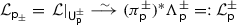Let ${\mathsf {U}}_ I \subset {\mathsf {X}}$ be a Stokes region with polar vertices $\mathsf {p}, \mathsf {p}' \in {\mathsf {D}}$, and let be the semilocal diagonal decomposition of ${{\mathcal {E}}}$ over ${\mathsf {U}}_ I $ (Proposition 2.46), where $\Lambda _i, \Lambda _{i'}$ are as in (14). Then there is a canonical flat isomorphism

(4)
.

Let ${\mathsf {U}}_i, {\mathsf {U}}_{i'}$ be the spectral regions above ${\mathsf {U}}_{ I }$ incident to $\mathsf {p}_-, \mathsf {p}'_- \in {\mathsf {C}}$, respectively, and recall the notation . Then there are canonical flat isomorphisms

(5)
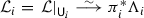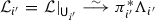and .

Finally, recall that $\eta $ is the canonical one-form on the spectral curve .

(6)
The abelian connection on the abelianisation line bundle ${{\mathcal {L}}}$ is holomorphic along ${\mathsf {C}}$; it has logarithmic poles only along the ramification divisor ${\mathsf {R}}$ with residues $-1/2$.

The following proposition, which readily follows from the discussion in Sect. 2.4, expresses the sense in which the abelianisation of connections is the analogue of abelianisation of Higgs bundles.

3.6 Proposition

(Spectral properties of abelianisation) For any simply connected open subset , the abelianisation line bundle ${{\mathcal {L}}}$ has a generator e which is an eigensection for with eigenvalue $\eta $ (in the sense of Sect. 2.4); i.e., it satisfies the following equation:

Moreover, over any spectral region , there is a canonical flat inclusion with respect to which this section e is an eigensection for $\pi ^*\nabla $ with eigenvalue $\eta $:

3.7 Example

Let us illustrate the above construction in the simplest possible explicit example. Consider a logarithmic $\mathfrak {sl}_2$-connection $({{\mathcal {E}}}, \nabla )$ from Example 2.5 with $d = 3$. Namely, ${\mathsf {X}} = \mathbb {P}^1$, ${{\mathcal {E}}} = {{\mathcal {O}}}_{\mathbb {P}^1}^{\oplus 2}$, and ${\mathsf {D}} \mathrel {\mathop :}=\left\{ 0, 1, \infty \right\} $. Let $ A _1, A _2$ be any pair of $\mathfrak {sl} (2, \mathbb {C})$-matrices, both with eigenvalues $\pm 1/3$, and let $\nabla $ be given by the formula (1). Then the $\nabla $ has Levelt exponents $\pm 1/3$ at each pole.

To abelianise $\nabla $, we must choose a generic saddle-free quadratic differential on $({\mathsf {X}}, {\mathsf {D}})$ with residues 1/9 at each point of ${\mathsf {D}}$. One such choice is the quadratic differential $\varphi _1$ from Example 2.22. Its spectral curve was described in Example 2.26, its Stokes and spectral graphs were detailed in Fig. 7, and the relevant Stokes open cover was presented in Fig. 8. Finally, in Fig. 11, we illustrate the abelianisation construction by displaying which Levelt line subbundle is considered on which Stokes and spectral region.

3.2 The Voros cocycle

This section introduces the main ingredient in constructing the deablianisation functor $\pi _\text {ab}^\Gamma $, the Voros cocycle. Let be its abelianisation of $({{\mathcal {E}}}, \nabla , M ) \in Conn _{\mathsf {X}}^2 (\Gamma )$.

3.8. The canonical nonabelian cocycle $ V $. Let ${\mathsf {U}}_\alpha \in \Gamma _1$ be a Stokes ray on ${\mathsf {X}}$ with polar vertex $\mathsf {p}\in {\mathsf {D}}$ and branch vertex $\mathsf {b}\in {\mathsf {B}}$. It is a component of the intersection of exactly two Stokes regions ${\mathsf {U}}_ I , {\mathsf {U}}_ J $ (see Fig. 12). Consider the pair of canonical identifications given by Proposition 3.5(4):

(24)

Over the Stokes ray ${\mathsf {U}}_{\alpha }$, their ratio yields a flat automorphism of :

(25)

where $\pi _* L $ denotes the associated local system on ${\mathsf {X}}^\circ $. The nerve of the cover $\mathfrak {{{U}}}_\Gamma $ of ${\mathsf {X}}^\circ $ consists of Stokes rays, so we obtain aČech 1-cocycle $ V $ with values in the local system $\mathcal {A}ut (\pi _* L )$:

(26)

3.9 Lemma

If $({{\mathcal {E}}}, \nabla , M ) \in Conn _{\mathsf {X}}^2 (\Gamma )$, let be its abelianisation, and consider the pushforward $\pi _*{{\mathcal {L}}} = \pi _*\pi ^\text {ab}_\Gamma {{\mathcal {E}}}$. If $ V $ is the cocycle (26), then there is a canonical isomorphism

Proof

The action of the cocycle $ V $ on the pushforward bundle $\pi _*{{\mathcal {L}}}$ is a new bundle ${{\mathcal {E}}}' \mathrel {\mathop :}= V \cdot \pi _*{{\mathcal {L}}}$. Explicitly, the local piece ${{\mathcal {E}}}'_{ I }$ over a Stokes region ${\mathsf {U}}_{ I }$ is defined to be , and the gluing data over a Stokes ray ${\mathsf {U}}_{\alpha } \subset {\mathsf {U}}_ I \cap {\mathsf {U}}_ J $ is given by $ V _{\alpha }$:

But this commutative square together with (24) and (25) imply that ${{\mathcal {E}}}$ and ${{\mathcal {E}}}'$ are canonically isomorphic. $\square $

3.10. Transposition paths. Let us explicitly compute each automorphism $ V _{\alpha }$ with respect to a pair of canonical decompositions of $\pi _*{{\mathcal {L}}}$ over the Stokes ray ${\mathsf {U}}_\alpha $. Through the isomorphisms and , the automorphism $ V _{\alpha } = \varphi _ J \circ \varphi _ I ^{-1}$ over ${\mathsf {U}}_\alpha $ is just the identity on ${{\mathcal {E}}}$ written as a map $\Lambda _i \oplus \Lambda _{i'} \rightarrow \Lambda _j \oplus \Lambda _{j'}$. Notice that $\Lambda _{i'} = \Lambda _{j'}$ because they are continuations of the same line bundle germ at $\mathsf {p}$, so using (16) we find:

(27)

Now, we can decompose the map $\Delta _\alpha : \Lambda _i \rightarrow \Lambda _{j'}$ through canonical inclusions, projections, and the upper-triangular expressions (16) for the identity on ${{\mathcal {E}}}$ as follows:

We interpret the first and second upper-triangular expressions as the identity maps on ${{\mathcal {E}}}$ over ${\mathsf {U}}_\gamma $ and ${\mathsf {U}}_\beta $, respectively. Since all these bundle maps are $\nabla $-flat, the map $\Delta _\alpha $ can be interpreted as the endomorphism of the fibre of ${{\mathcal {E}}}$ over a point in ${\mathsf {U}}_\alpha $ obtained as the composition of $\nabla $-parallel transports $ P _ I , P _ K , P _ J $ along paths $\delta _ I $ contained in ${\mathsf {U}}_ I $ from ${\mathsf {U}}_\alpha $ to ${\mathsf {U}}_\gamma $, followed by $\delta _ K $ contained in ${\mathsf {U}}_ K $ from ${\mathsf {U}}_\gamma $ to ${\mathsf {U}}_\beta $, followed by $\delta _ J $ contained in ${\mathsf {U}}_ J $ from ${\mathsf {U}}_\beta $ back to ${\mathsf {U}}_\alpha $ (see Fig. 12).

Explicitly:

The key idea, which goes back to Gaiotto–Moore–Neitzke [8], is to notice that this expression has an interpretation as a parallel transport for the abelian connection on the spectral curve. Indeed, if we fix points $\mathsf {p}, \mathsf {p}', \mathsf {p}''$ in ${\mathsf {U}}_\alpha , {\mathsf {U}}_\gamma , {\mathsf {U}}_\beta $ as shown in Fig. 12, then through the canonical identification of fibres using Proposition 3.5(4), we have:

Here, $\Delta ^+_\alpha $ is defined by the diagram; we used (22), and $p_i, p_k, p_{j'}$ are -parallel transports along the paths $\delta _i, \delta _k, \delta _{j'}$ which are the lifts of $\delta _ I , \delta _ K , \delta _ J $ as shown in Fig. 12. Since $g^+_{\beta }, g^-_{\gamma }$ are precisely the gluing maps for ${{\mathcal {L}}}$, we find that $\Delta ^+_\alpha $ is nothing but the parallel transport of along the clockwise semicircular path $\delta _\mathsf {p}^+ \mathrel {\mathop :}=\delta _{j'} \delta _k \delta _{i}$ (our paths compose the same way as maps: from right to left) around the ramification point $\mathsf {r}$ starting at $\mathsf {p}_+$ and ending at $\mathsf {p}_-$. The Stokes graph determines such sheet transposition paths on all Stokes rays: i.e., for any $\mathsf {p}\in {\mathsf {U}}_\alpha $, the path $\delta _\mathsf {p}^+$ on is the unique lift starting at $\mathsf {p}_+$ of a clockwise loop $\delta _\mathsf {p}$ based at $\mathsf {p}\in {\mathsf {U}}_\alpha $ around the branch point $\mathsf {b}$ (see Fig. 13).

3.11 Lemma

For every Stokes ray ${\mathsf {U}}_\alpha \subset {\mathsf {X}}$ and every point $\mathsf {p}\in {\mathsf {U}}_{\alpha }$, the automorphism $ V _{\alpha , \mathsf {p}}$ of the fibre is:

(28)

The correspondence $\mathsf {p}_+ \mapsto \delta ^+_{\mathsf {p}}$ is a well-defined map , where is the fundamental groupoid of the punctured spectral curve, which is the set of paths on considered up to homotopy with fixed endpoints. If we define a flat bundle isomorphism

then $\Delta _\alpha = \pi _*\Delta ^+_\alpha $ defines an endomorphism of $\pi _*{{\mathcal {L}}}$ over the Stokes ray ${\mathsf {U}}_{\alpha }$. So Lemma 3.11 may be expressed in terms of bundle maps as follows.

3.12 Lemma

For every $\alpha \in \Gamma _1$, the automorphism $ V _{\alpha }$ of is $ V _{\alpha } = \text {id}+ \pi _*\Delta ^+_\alpha $.

3.13. The Voros cocycle. One of the central observations in this paper is that formula (28) does not depend on the fact that is the abelianisation of $({{\mathcal {E}}}, \nabla )$. Indeed, this formula is written purely in terms of the parallel transport along canonically defined paths on and the pushforward functor $\pi _*$. In other words, if is any abelian connection (i.e., not a priori the abelianisation of some connection on ${\mathsf {X}}$), then for each Stokes ray $\alpha \in \Gamma _1$, we can consider the automorphism $ V _{\alpha }$ of $\pi _*{{\mathcal {L}}}$ over ${\mathsf {U}}_{\alpha }$ defined by

(29)

for each $\mathsf {p}\in {\mathsf {U}}_{\alpha }$ with preimages $\mathsf {p}_\pm \in {\mathsf {U}}_{\alpha }^\pm $. As a bundle automorphism over ${\mathsf {U}}_{\alpha }$,

(30)

where and . This yields a cocycle

(31)

Now, if is a morphism in , and $ V , V '$ are respectively the cocycles for ${{\mathcal {L}}}, {{\mathcal {L}}}'$ defined by the formula (29), then the identity immediately implies the following commutative square for every $\alpha $:

(32)

In other words, for every Stokes ray $\alpha \in \Gamma _1$, the collection

(33)

indexed by abelian connections , forms a natural transformation

of the pushforward functor (2), defined over ${\mathsf {U}}_{\alpha }$. We obtain a cocycle valued in the local system $\mathcal {A}ut (\pi _*)$ of nonabelian groups on the punctured base curve ${\mathsf {X}}^\circ $ consisting of natural automorphisms of $\pi _*$.

3.14 Definition

(Voros cocycle) The Voros cocycle is the nonabelian Čech 1-cocycle

$\square $

3.15. Abelianisation of the Voros cocycle. The parallel transports $\Delta _\alpha $ can also be arranged into a cocycle as follows. If is any abelian connection, then , where and for each $\alpha \in \Gamma ^+_1$. The sheaf $\mathcal {H}om ( L , \sigma ^* L )$ is a local system of abelian groups, and we can define an abelian Čech 1-cocycle on by

(34)

by and is a morphism in , and $\Delta , \Delta '$ are the corresponding cocycles, then the identity implies for every $\alpha $ a pair of commutative squares:

(35)

In other words, for every $\alpha $, the collection of flat homomorphisms

indexed by abelian connections , forms a natural transformation

defined over ${\mathsf {U}}_{\alpha }^\pm $. Here, is the pullback functor by the canonical involution $\sigma $. Thus, we obtain a cocycle valued in the local system $\mathcal {H}om (\text {id}, \sigma ^*)$ of abelian groups on the punctured spectral curve consisting of natural transformations from the identity functor $\text {id}$ to the pullback functor $\sigma ^*$:

(36)

Formula (30) makes it apparent that the Voros cocycle $\mathbb {V}$ is completely determined by the cocycle ; let us make this precise. Suppose , and choose a point $\mathsf {p}\in {\mathsf {U}}_{\alpha }$ for some $\alpha $. If $\mathsf {p}_\pm \in {\mathsf {U}}_{\alpha }^\pm $ are the two preimages of $\mathsf {p}$, then the canonical isomorphism on stalks induces a canonical inclusion of $\mathcal {H}om ( L , \sigma ^* L )_{\mathsf {p}_\pm }$ into ${\mathcal {End}} (\pi _* L )_\mathsf {p}$ via

Given any $c \in \mathcal {H}om ( L , \sigma ^* L )_{\mathsf {p}_\pm }$, we denote its image in $\mathcal {E}nd (\pi _* L )_\mathsf {p}$ by $\pi _*c$.

3.16 Proposition

The Voros cocycle $\mathbb {V}$ and the abelian cocycle satisfy , where is the identity cocycle.

That is to say, the nonabelian Voros cocycle $\mathbb {V}$ is actually ‘in disguise’ the data of an abelian cocycle but on a different curve. In other words, should be thought of as the abelianisation of the Voros cocycle.

Proof

Notice that $\pi $ induces a double cover , yielding a map on cocycles:

(37)

Then formula (30) implies that $\mathbb {V}$ is the image of . $\square $

3.3 The nonabelianisation functor

In this section, we construct the nonabelianisation functor $\pi _\text {ab}^\Gamma $ and prove that it is an inverse equivalence to the abelianisation functor $\pi _\Gamma ^\text {ab}$. The main ingredient is the Voros cocycle $\mathbb {V}$, and the construction proceeds in two steps. If is an abelian connection on , we first use the the pushforward functor $\pi _*$ to obtain a rank-two connection on $({\mathsf {X}}, {\mathsf {D}} \cup {\mathsf {B}})$. But does not holomorphically extend over the branch locus ${\mathsf {B}}$, because it has nontrivial monodromy around ${\mathsf {B}}$, as we remarked after the proof of Proposition 2.15. Therefore, $\pi _*$ cannot invert $\pi ^\text {ab}_\Gamma $, because its image is not even contained in $Conn _{\mathsf {X}}^2$. Instead, step two is to use the Voros cocycle $\mathbb {V}$ to deform $\pi _*$ as a functor. The result is the nonabelianisation functor $\pi _\text {ab}^\Gamma $.

3.17. Construction of $\nabla $. Given any abelian connection , we construct $({{\mathcal {E}}}, \nabla , M ) \in Conn _{\mathsf {X}}^2 (\Gamma )$. Consider the pushforward . The Voros cocycle $\mathbb {V}$ determines a cocycle $ V \mathrel {\mathop :}=\mathbb {V}({{\mathcal {L}}}) \in {\check{Z}}^1 \big (\mathfrak {{{U}}}_\Gamma , \mathcal {A}ut (\pi _*{{\mathcal {L}}}) \big )$.

Definition over Stokes regions. The main step in the construction is to use $ V $ to reglue $\pi _*{{\mathcal {L}}}$ over Stokes rays. For each Stokes region ${\mathsf {U}}_ I $, let

and if ${\mathsf {U}}_\alpha $ is a Stokes ray in the ordered double intersection ${\mathsf {U}}_ I \cap {\mathsf {U}}_ J $, then the gluing over ${\mathsf {U}}_\alpha $ is given by . If ${\mathsf {U}}_i$ is a spectral region in the preimage of ${\mathsf {U}}_ I $, then since ${{\mathcal {E}}}_ I ({\mathsf {U}}_ I ) = {{\mathcal {L}}} ({\mathsf {U}}_i) \oplus \sigma ^*{{\mathcal {L}}} ({\mathsf {U}}_i)$, the map $ M _ I $ defines an $\mathfrak {sl}_2$-structure on each local piece ${{\mathcal {E}}}_{ I }$. Moreover, $ M _ I $ and $ M _ J $ glue over ${\mathsf {U}}_\alpha $ because $ V _{\alpha }$ is unipotent with respect to the corresponding decompositions.

Definition at the poles. Recall that the infinitesimal punctured disc ${\mathsf {U}}_\mathsf {p}^*$ centred at a point $\mathsf {p}\in {\mathsf {D}}$ is covered by sectorial neighbourhoods coming from the Stokes regions incident to $\mathsf {p}$. Thanks to the upper-triangular nature of the Voros cocycle $ V $, we obtain a flat bundle ${{\mathcal {E}}}_\mathsf {p}^*$ over ${\mathsf {U}}_\mathsf {p}^*$ equipped with a filtration $({{\mathcal {E}}}_\mathsf {p}^*)^\bullet $ whose associated graded is canonically isomorphic to . Now, it is a simple fact that if the associated graded of a filtered connection extends over a point, then the filtered connection itself extends with the same Levelt exponents. Thus, ${{\mathcal {E}}}_\mathsf {p}^*$ has a canonical extension over ${\mathsf {U}}_\mathsf {p}$ to a bundle ${{\mathcal {E}}}_\mathsf {p}$ with connection $\nabla _\mathsf {p}$ that has logarithmic poles at $\mathsf {p}$ and Levelt exponents $\pm \lambda _\mathsf {p}$. It remains to define $\nabla $ over the branch locus ${\mathsf {B}}$.

Definition at the branch points. We will first compute the monodromy of $\nabla $ around each branch point directly to show that it is trivial, and then use Deligne’s canonical extension [5, pp. 91–96].

3.18 Lemma

The monodromy of $\nabla $ around any branch point is trivial. Therefore, the connection $({{\mathcal {E}}}, \nabla , M )$ on ${\mathsf {X}}^\circ $ has a canonical holomorphic extension over ${\mathsf {B}}$.

The technique is to express the parallel transport of $\nabla $ along paths on ${\mathsf {X}}$ in terms of the parallel transport of along their lifts to as well as the sheet transposition paths. We adopt the following notation for the parallel transports of , respectively:

It follows immediately from the construction of ${{\mathcal {E}}}$ that if $\wp $ is a path on ${\mathsf {X}}^\circ $ contained in a Stokes region, then $ P (\wp ) = \pi _*p (\wp )$. Explicitly, let $\wp ', \wp ''$ be the two lifts of $\wp $ to . Let $\mathsf {x}, \mathsf {y}$ be the startpoint and the endpoint of $\wp $, and similarly for $\wp ', \wp ''$. Then, for example, the fibre is the direct sum of fibres $L_{\mathsf {x}'} \oplus L_{\mathsf {x}''}$ of ${{\mathcal {L}}}$. With respect to these decompositions, the parallel transport $ P (\wp ) : E_{\mathsf {x}} \longrightarrow E_{\mathsf {y}}$ is expressed as

(38)

We say that a path $\wp $ on ${\mathsf {X}}^\circ $ (or ) is a short path if its endpoints do not belong to the Stokes graph $\Gamma $ (or to the spectral graph ) and it intersects at most one Stokes ray (or spectral ray). If $\wp $ is a short path on ${\mathsf {X}}^\circ $ that intersects a Stokes ray ${\alpha } \in \Gamma _1$, then $\wp $ is divided into two segments $\wp _-, \wp _+$ (Fig. 14).

Each $\wp _\pm $ is contained in a Stokes region, so $ P (\wp _\pm ) = \pi _*p (\wp _\pm )$. On the other hand, the vector bundle ${{\mathcal {E}}}$ is constructed by gluing $\pi _*{{\mathcal {L}}}$ to itself over ${\mathsf {U}}_{\alpha }$ by the automorphism $ V _{\alpha }$, so we obtain the following formula for $ P (\wp )$:

(39)

Explicitly, let $\wp ', \wp ''$ denote the two lifts of $\wp $ to , where $\wp '$ intersects $\alpha _-$ and $\wp ''$ intersects $\alpha _+$ (Fig. 14). The parallel transport $ P (\wp ) : E_{\mathsf {x}} \longrightarrow E_{\mathsf {y}}$ can be expressed as

The off-diagonal term $p (\wp '_+) \Delta _{\alpha }^+ p (\wp ''_-)$ is the parallel transport of along the concatenated path $\wp ^+_\alpha \mathrel {\mathop :}=\wp '_+ \delta ^+_\alpha \wp ''_-$ (Fig. 15), so

(40)

Proof of Lemma 3.18

Fix a branch point $\mathsf {b}\in {\mathsf {B}}$, and let ${\mathsf {U}}_{\alpha }, {\mathsf {U}}_{\beta }, {\mathsf {U}}_{\gamma }$ be the three Stokes rays incident to $\mathsf {b}$. Fix a basepoint $\mathsf {x}$ in the Stokes region ${\mathsf {U}}_ I $ as shown in Fig. 16, and also fix a loop $\wp $ around $\mathsf {b}$. We calculate the monodromy $ P (\wp )$. Fix two more basepoints $\mathsf {y}, \mathsf {z}$ in the other two Stokes regions, thus dividing the loop $\wp $ into three short paths denoted by $\wp _\alpha , \wp _\beta , \wp _\gamma $, as explained in Fig. 17. Then $ P (\wp ) = P (\wp _\gamma ) P (\wp _\beta ) P (\wp _\alpha )$. Each $ P (\wp _\bullet )$ (where $\bullet = \alpha , \beta , \gamma $) can be expressed via (39) as

Now, let $\wp ', \wp ''$ be the two lifts of $\wp $ to , as explained in Fig. 18. The lifts $\wp ''_\alpha , \wp '_\beta , \wp ''_\gamma $ intersect the positive spectral rays $\alpha _+, \beta _+, \gamma _+$, giving rise to three sheet transposition paths $\wp ^+_\alpha , \wp ^+_\beta , \wp ^+_\gamma $ as shown in Fig. 19. By inspection,

(41)

The explicit formula (40) gives three expressions:

Notice that $ P (\wp _\beta )$ is lower-triangular in the given decompositions of and , because it is the lift $\wp '_\beta $ of $\wp _\beta $ starting at $\mathsf {y}'$ that intersects the positive spectral ray $\beta _+$. Also notice that the source fibre of $ P (\wp _\alpha )$ is decomposed as $L_{\mathsf {x}'} \oplus L_{\mathsf {x}''}$, whilst the target fibre of $ P (\wp _\gamma )$ is decomposed as $L_{\mathsf {x}''} \oplus L_{\mathsf {x}'}$, so the monodromy $ P (\wp ) \in {\mathsf {Aut}}\big (L_{\mathsf {x}'} \oplus L_{\mathsf {x}''} \big )$ is given by

Applying relations (41), we find that $\wp ''_\gamma \wp ^+_{\beta } \wp '_\alpha = \wp ''_\gamma (\wp '_\alpha \wp ''_\gamma )^{-1} \wp '_\alpha = 1$, which is a constant path at $\mathsf {x}'$, so the top-left entry of $ P (\wp )$ is 1. Next, the path $\wp ^+_{\gamma } \wp ^+_{\beta } \wp '_\alpha $ appearing in the bottom-left entry, simplifies to $(\wp ''_\gamma \wp ''_\beta \wp ''_\alpha )^{-1}$, so $p(\wp ^+_{\gamma } \wp ^+_{\beta } \wp ^+_{\alpha }) = p (\wp '_\gamma \wp '_\beta \wp '_\alpha )^{-1}$. Now, $\wp ''_\gamma \wp ''_\beta \wp ''_\alpha \wp '_\gamma \wp '_\beta \wp '_\alpha $ is a loop around the ramification point $\mathsf {r}$ based at $\mathsf {x}'$, and since the connection has monodromy $-1$ around $\mathsf {r}$ by Proposition 2.12, we find:

It follows that $p (\wp '_\gamma \wp '_\beta \wp '_\alpha )^{-1} = - p (\wp ''_\gamma \wp ''_\beta \wp ''_\alpha )$, and so the bottom-left entry of $ P (\wp )$ is 0. Similarly, we can calculate the other entries of $ P (\wp )$ and find that $ P (\wp ) = \text {id}$. $\square $

3.19. Diagonal decompositions and transversality. The fact that the connection $\nabla $ is transverse with respect to $\Gamma $ is deduced from the fact that the local and semilocal diagonal decompositions of ${{\mathcal {E}}}$ (Propositions 2.8 and 2.46) can be easily recovered from our construction as follows. Let ${\mathsf {U}}_\mathsf {p}$ be the infinitesimal disc around a pole $\mathsf {p}\in {\mathsf {D}}$. If ${\mathsf {U}}_\mathsf {p}^\pm $ are respectively the infinitesimal discs around $\mathsf {p}_\pm $, let and $\Lambda _\mathsf {p}^\pm \mathrel {\mathop :}=\pi _*{{\mathcal {L}}}_\mathsf {p}^\pm $. Then it follows from the construction of ${{\mathcal {E}}}$ over ${\mathsf {U}}_\mathsf {p}$ that the local diagonal decomposition of ${{\mathcal {E}}}_\mathsf {p}$ is precisely . As a result, the local Levelt filtration of ${{\mathcal {E}}}$ at $\mathsf {p}$ is ${{\mathcal {E}}}_\mathsf {p}^\bullet = \big ( \Lambda _\mathsf {p}^- \subset {{\mathcal {E}}}^\mathsf {p}\big )$.

Let ${\mathsf {U}}_ I $ be a Stokes region with $ I = \left\{ i,i' \right\} $ and with polar vertices $\mathsf {p}, \mathsf {p}'$ such that the spectral regions ${\mathsf {U}}_i, {\mathsf {U}}_{i'}$ are respectively incident to the preimages $\mathsf {p}_-, \mathsf {p}'_-$. By construction, if and $\smash {\Lambda _{i^{(\prime )}} \mathrel {\mathop :}=\pi _*{{\mathcal {L}}}_{i^{(\prime )}}}$, then ${{\mathcal {E}}}_ I = \Lambda _i \oplus \Lambda _{i'}$. Of course, ${{\mathcal {L}}}_{i}$ is the unique continuation of ${{\mathcal {L}}}_{\mathsf {p}}^-$ from ${\mathsf {U}}_{\mathsf {p}}^-$ to ${\mathsf {U}}_i$, and therefore $\Lambda _i$ is the unique continuation of $\Lambda _\mathsf {p}^-$ from ${\mathsf {U}}_\mathsf {p}$ to ${\mathsf {U}}_ I $. Same for $\Lambda _{i'}$. As a result, the direct sum $\Lambda _i \oplus \Lambda _{i'}$ is nothing but the transverse intersection ${{\mathcal {E}}}_{\mathsf {p}, I }^\bullet \pitchfork {{\mathcal {E}}}_{\mathsf {p}', I }^\bullet $ of Levelt filtrations ${{\mathcal {E}}}_\mathsf {p}^\bullet , {{\mathcal {E}}}_{\mathsf {p}'}^\bullet $ continued to ${\mathsf {U}}_ I $. This demonstrates the fact that $\nabla $ is transverse with respect to $\Gamma $, so $({{\mathcal {E}}}, \nabla , M ) \in Conn _{\mathsf {X}}^2 (\Gamma )$.

3.20 Proposition

The correspondence extends to a functor

This follows immediately from the commutative square (32). We call $\pi _\text {ab}^\Gamma $ the nonabelianisation functor, and the image under $\pi _\text {ab}^\Gamma $ the nonabelianisation of with respect to the Stokes graph $\Gamma $. Finally, our Main Theorem 3.3 follows from the following proposition.

3.21 Proposition

The functors $\pi ^\text {ab}_\Gamma , \pi _\text {ab}^\Gamma $ form a pair of inverse equivalences of categories.

Proof

Given $({{\mathcal {E}}}, \nabla , M ) \in Conn _{\mathsf {X}}^2 (\Gamma )$, let be its image under $\pi ^\text {ab}_\Gamma $. By construction, the Voros cocycle $\mathbb {V}$ applied to ${{\mathcal {L}}}$ is the cocycle $ V $ from (26). Lemma 3.9 gives a canonical isomorphism , so $\pi _\text {ab}^\Gamma \pi ^\text {ab}_\Gamma \Rightarrow \text {Id}$.

The converse is clear from the discussion above of diagonal decompositions and transversality (3.3), so we will be brief. Given , let $({{\mathcal {E}}}, \nabla , M )$ in $Conn _{\mathsf {X}}^2 (\Gamma )$ be its nonabelianisation, and suppose ${{\mathcal {L}}}'$ is the abelianisation of ${{\mathcal {E}}}$. First, we have for every $\mathsf {p}\in {\mathsf {D}}$. If is a spectral region with sink polar vertex $\mathsf {p}_-$, then $\Lambda _i = \pi _*{{\mathcal {L}}}_i$ is the unique continuation of $\Lambda _\mathsf {p}^-$. Both ${{\mathcal {L}}}_i$ and ${{\mathcal {L}}}'_i$ are the unique continuations of $(\pi _\mathsf {p}^-)^*\Lambda _\mathsf {p}^-$ to ${\mathsf {U}}_i$, we get . Thus, ${{\mathcal {L}}}, {{\mathcal {L}}}'$ are canonically isomorphic over , and because their extensions over ${\mathsf {R}}$ are unique, this isomorphism also extends over . So , and hence $\text {id}\Rightarrow \pi ^\text {ab}_\Gamma \pi _\text {ab}^\Gamma $. $\square $

References

Beauville, A., Narasimhan, M.S., Ramanan, S.: Spectral curves and the generalised theta divisor. J. Reine Angew. Math. 398, 169–179 (1989)
MathSciNet MATH Google Scholar
Borel, A., Grivel, P.-P., Kaup, B., Haefliger, A., Malgrange, B., Ehlers, F.: Algebraic $D$-Modules. Perspectives in Mathematics, vol. 2. Academic Press Inc., Boston (1987)
Google Scholar
Bridgeland, T., Smith, I.: Quadratic differentials as stability conditions. Publ. Math. Inst. Hautes Études Sci. 121, 155–278 (2015)
Article MathSciNet Google Scholar
Delabaere, É., Dillinger, H., Pham, F.: Résurgence de Voros et périodes des courbes hyperelliptiques. Ann. Inst. Fourier (Grenoble) 43(1), 163–199 (1993)
Article MathSciNet Google Scholar
Deligne, P.: Équations différentielles à points singuliers réguliers. Lecture Notes in Mathematics, vol. 163. Springer, Berlin (1970)
Esnault, H., Viehweg, E.: Logarithmic De Rham complexes and vanishing theorems. Invent. Math. 86, 161 (1986)
Article MathSciNet Google Scholar
Gabella, M.: Quantum holonomies from spectral networks and framed BPS states. Commun. Math. Phys. 351(2), 563–598 (2017)
Article MathSciNet Google Scholar
Gaiotto, D., Moore, G.W., Neitzke, A.: Spectral networks. Ann. Henri Poincaré 14(7), 1643–1731 (2013)
Article MathSciNet Google Scholar
Gaiotto, D., Moore, G.W., Neitzke, A.: Wall-crossing, Hitchin systems, and the WKB approximation. Adv. Math. 234, 239–403 (2013)
Article MathSciNet Google Scholar
Gaiotto, D., Moore, G.W., Neitzke, A.: Spectral networks and snakes. Ann. Henri Poincaré 15(1), 61–141 (2014)
Article MathSciNet Google Scholar
Gualtieri, M., Li, S., Pym, B.: The Stokes groupoids. J. Reine Angew. Math. 739, 81–119 (2018)
Article MathSciNet Google Scholar
Hausel, T., Pauly, C.: Prym varieties of spectral covers. Geom. Topol. 16(3), 1609–1638 (2012)
Article MathSciNet Google Scholar
Hitchin, N.J.: The self-duality equations on a Riemann surface. Proc. London Math. Soc. 55(1), 59–126 (1987). https://doi.org/10.1112/plms/s3-55.1.59
Hollands, L., Neitzke, A.: Spectral networks and Fenchel–Nielsen coordinates. Lett. Math. Phys. 106(6), 811–877 (2016)
Article MathSciNet Google Scholar
Hubbard, J., Masur, H.: Quadratic differentials and foliations. Acta Math. 142(3–4), 221–274 (1979)
Article MathSciNet Google Scholar
Kawai, T., Takei,Y.: Algebraic analysis of singular perturbation theory. Translations of Mathematical Monographs, vol. 227. American Mathematical Society, Providence (2005). Translated from the 1998 Japanese original by Goro Kato, Iwanami Series in Modern Mathematics
Korotkin, D.: Solution of matrix Riemann–Hilbert problems with quasi-permutation monodromy matrices. Math. Ann. 329(2), 335–364 (2004)
Article MathSciNet Google Scholar
Levelt, A.H.M.: Hypergeometric functions. Doctoral thesis, University of Amsterdam. Drukkerij Holland N. V., Amsterdam (1961)
Nikolaev, N.: Abelianisation of logarithmic connections. Ph.D. thesis, University of Toronto (2018)
Strebel, K.: Quadratic Differentials. Ergebnisse der Mathematik und ihrer Grenzgebiete (3) [Results in Mathematics and Related Areas (3)], vol. 5. Springer, Berlin (1984)
Google Scholar
Voros, A.: The return of the quartic oscillator. The complex WKB method. Ann l’I.H.P. Phys. théorique 39(3), 211–338 (1983)
Wasow,W.: Asymptotic expansions for ordinary differential equations. Robert E. Krieger Publishing Co., Huntington (1976). Reprint of the 1965 edition

Download references

Acknowledgements

The author thanks Francis Bischoff, Aaron Fenyes, Alberto García-Raboso, Kohei Iwaki, Omar Kidwai, Andrew Neitzke, Steven Rayan, and Shinji Sasaki for helpful and enlightening discussions. Many thanks also go to the anonymous referee for their very thoughtful and helpful comments. The author expresses special gratitude to Marco Gualtieri, who suggested the problem and provided so much invaluable input, support, and encouragement as the author’s thesis advisor. At various stages, this work was supported by the Ontario Graduate Scholarship and by the NCCR SwissMAP of the SNSF.

Author information

Authors and Affiliations

School of Mathematics and Statistics, University of Sheffield, Sheffield, UK
Nikita Nikolaev

Authors

Nikita Nikolaev
View author publications
You can also search for this author in PubMed Google Scholar

Corresponding author

Correspondence to Nikita Nikolaev.

Additional information

Publisher's Note

Springer Nature remains neutral with regard to jurisdictional claims in published maps and institutional affiliations.

Rights and permissions

Open Access This article is licensed under a Creative Commons Attribution 4.0 International License, which permits use, sharing, adaptation, distribution and reproduction in any medium or format, as long as you give appropriate credit to the original author(s) and the source, provide a link to the Creative Commons licence, and indicate if changes were made. The images or other third party material in this article are included in the article’s Creative Commons licence, unless indicated otherwise in a credit line to the material. If material is not included in the article’s Creative Commons licence and your intended use is not permitted by statutory regulation or exceeds the permitted use, you will need to obtain permission directly from the copyright holder. To view a copy of this licence, visit http://creativecommons.org/licenses/by/4.0/.

Reprints and permissions

About this article

Cite this article

Nikolaev, N. Abelianisation of logarithmic $\mathfrak {sl}_2$-connections. Sel. Math. New Ser. 27, 78 (2021). https://doi.org/10.1007/s00029-021-00688-5

Download citation

Accepted: 30 June 2021
Published: 03 August 2021
DOI: https://doi.org/10.1007/s00029-021-00688-5

Keywords

Mathematics Subject Classification

Use our pre-submission checklist

Avoid common mistakes on your manuscript.

Abelianisation of logarithmic \(\mathfrak {sl}_2\)-connections

Abstract

Similar content being viewed by others

Lie groupoids and logarithmic connections

The locus of the representation of logarithmic connections by Fuchsian equations

Differential characters and cohomology of the moduli of flat connections

1 Introduction

1.1 Main result

1.2 Context: spectral networks and exact WKB

1.3 Outlook

1.4 Content

2 Logarithmic connections and spectral curves

2.1 Logarithmic connections and Levelt filtrations

2.3 Definition

2.5 Example

2.8 Proposition

2.9 Example

2.2 Logarithmic connections and double covers

2.11 Definition

2.12 Proposition

Proof

2.13 Proposition

2.15 Proposition

Proof

2.3 Spectral curves for quadratic differentials

2.18 Lemma

Proof

2.21 Lemma

2.22 Example

2.24 Example

2.26 Example

2.4 Logarithmic connections and spectral curves

2.5 The Stokes graph

2.34 Example

2.36 Definition

2.38 Example

2.42 Example

2.6 Transverse connections

2.45 Definition

2.46 Proposition

2.48 Remark

3 Abelianisation

3.3 Theorem

3.1 The abelianisation functor

3.4 Proposition

3.5 Proposition

3.6 Proposition

3.7 Example

3.2 The Voros cocycle

3.9 Lemma

Proof

3.11 Lemma

3.12 Lemma

3.14 Definition

3.16 Proposition

Proof

3.3 The nonabelianisation functor

3.18 Lemma

Proof of Lemma 3.18

3.20 Proposition

3.21 Proposition

Proof

References

Acknowledgements

Author information

Authors and Affiliations

Corresponding author

Additional information

Publisher's Note

Rights and permissions

About this article

Cite this article

Share this article

Keywords

Mathematics Subject Classification

Search

Navigation