The pure cohomology of multiplicative quiver varieties

Abstract

To a quiver Q and choices of nonzero scalars $q_i$, non-negative integers $\alpha _i$, and integers $\theta _i$ labeling each vertex i, Crawley-Boevey–Shaw associate a multiplicative quiver variety ${\mathcal {M}}_\theta ^q(\alpha )$, a trigonometric analogue of the Nakajima quiver variety associated to Q, $\alpha$, and $\theta$. We prove that the pure cohomology, in the Hodge-theoretic sense, of the stable locus ${\mathcal {M}}_\theta ^q(\alpha )^{{\text {s}}}$ is generated as a ${\mathbb {Q}}$-algebra by the tautological characteristic classes. In particular, the pure cohomology of genus g twisted character varieties of $GL_n$ is generated by tautological classes.

1 Introduction

A quiver $Q=(I,\Omega )$ is a directed graph with vertex set I and edge set $\Omega$. Despite its simple definition, from the datum of a quiver one can build, using various geometric quotient constructions, rich families of symplectic algebraic varieties. The best-known examples of this are [25] Nakajima’s quiver varieties. In this paper, however, we will study their cousins, the multiplicative quiver varieties, first introduced by Crawley-Boevey and Shaw [10]. Just as Nakajima’s quiver varieties can be understood as (coarse) moduli spaces of semistable representations of a class of algebras known as preprojective algebras their multiplicative analogues can be viewed similarly as moduli spaces of representations of a noncommutative algebra $\Lambda ^q$, the multiplicative preprojective algebra.

The significance of multiplicative quiver varieties is rapidly growing: Crawley-Boevey and Shaw were led to them through their work on the celebrated Deligne–Simpson problem. Subsequently they have been shown to arise as moduli spaces of irregular connections in the work [3, 4] of Boalch and Yamakawa (indeed Boalch’s work [3] lead him to define an even more general notion of multiplicative quiver variety than that considered here). Bezrukavnikov and Kapranov [2] realise them as moduli of microlocal sheaves on nodal curves (see also the work of Crawley-Boevey [11]), while in symplectic topology the work of Etgü and Lekili [15] shows that the Fukaya categories of certain symplectic four-manifolds, which are built from quiver-type data, are controlled by a derived version of the associated multiplicative preprojective algebra. Moreover, results of Chalykh and Fairon [7] and Braverman–Etingof–Finkelberg [5] reveal exciting new connections between multiplicative quiver varieties and new families of integrable systems which have also been constructed using double affine Hecke algebras.

Recently a number of authors [27, 30] have studied the geometry of multiplicative quiver varieties. The present paper is a contribution to the study of their topology, and, as we discuss later, we expect its results will help shed light on questions raised by Hausel and collaborators in [20].

1.1 Results

Just as for a Nakajima quiver variety, a multiplicative quiver variety ${\mathcal {M}}_{\theta }^q(\alpha )$, where $\alpha \in {\mathbb {N}}^I$ is a dimension vector, is defined as a GIT quotient (at a character $\chi _\theta : {\mathbb {G}}\rightarrow {{\mathbb {G}}}_m$) of the affine algebraic variety ${\text {Rep}}(\Lambda ^q,\alpha )$ of (framed) representations of $\Lambda ^q(\alpha )$ by the group ${\mathbb {G}} = \big (\prod _i GL(\alpha _i)\big )/\Delta ({{\mathbb {G}}}_m)$, a product of general linear groups modulo the diagonal copy of ${{\mathbb {G}}}_m$; when it is a free quotient, this endows ${\mathcal {M}}_{\theta }^q(\alpha )$ with a map $c:{\mathcal {M}}_{\theta }^q(\alpha )\rightarrow B{\mathbb {G}}$.

The rational cohomology $H^*(B{\mathbb {G}},{\mathbb {Q}})$ is pure in the sense of Hodge theory: $H^m(B{\mathbb {G}},{\mathbb {Q}}) = W_mH^m(B{\mathbb {G}},{\mathbb {Q}})$ and $W_{m-1}H^mB{\mathbb {G}},{\mathbb {Q}}))=0$, where $W_kH^m(B{\mathbb {G}},{\mathbb {Q}})$ denotes the k-th piece of the weight filtration.

It follows that if we set

$$\begin{aligned} PH^*({\mathcal {M}}_{\theta }^q(\alpha )) \overset{{\text {def}}}{=} \displaystyle \bigoplus _m \mathrm {gr}W_m\big (H^m\big ({\mathcal {M}}_{\theta }^q(\alpha ), {\mathbb {Q}}\big )\big ), \end{aligned}$$

to be the “pure part” of the cohomology, where $\text {gr}W$ denotes the associated graded with respect to the weight filtration, then the image of the pullback map $c^*$ on cohomology must inject into the pure part of the cohomology of ${\mathcal {M}}_{\theta }^q(\alpha )$.

Remark 1.1

Note that for a smooth variety X the weight filtration on $H^m(X,{\mathbb {Q}})$ vanishes below degree m, so that $\text {gr}W_m(H^m(X,{\mathbb {Q}})) = W_m(H^m(X,{\mathbb {Q}}))$. Thus for such spaces the pure part of cohomology is a subspace of the ordinary cohomology.

The main result of the present paper is:

Theorem 1.2

• (1) Suppose that $U\subseteq {\mathcal {M}}_{\theta }^q(\alpha )^{{\text {s}}}$ is any connected open subset of the stable locus of the multiplicative quiver variety ${\mathcal {M}}_{\theta }^q(\alpha )$. Then the induced map on cohomology

  $$\begin{aligned} H^*(B{\mathbb {G}}, {\mathbb {Q}})\rightarrow H^*\big (U, {\mathbb {Q}}\big ) \end{aligned}$$

  defines a surjection onto the pure cohomology $PH^*(U) = \displaystyle \bigoplus _m \mathrm {gr}W_m\big (H^m\big (U, {\mathbb {Q}}\big )\big )$.

• (2) In particular, if ${\mathcal {M}}_{\theta }^q(\alpha ) = {\mathcal {M}}_{\theta }^q(\alpha )^{{\text {s}}}$ and ${\mathcal {M}}_{\theta }^q(\alpha )$ is connected, then

  $$\begin{aligned} H^*(B{\mathbb {G}}, {\mathbb {Q}})\rightarrow H^*\big ({\mathcal {M}}_{\theta }^q(\alpha ), {\mathbb {Q}}\big ) \end{aligned}$$

  surjects onto $PH^*\big ({\mathcal {M}}_{\theta }^q(\alpha )\big )$.

In light of Theorem 1.2 of [26], Theorem 1.2 is nicely consonant with Hausel’s “purity conjecture” (cf. [17] as well as [19, Theorem 1.3.1 and Corollary 1.3.2], and the discussion around Conjecture 1.1.3 of [20]), which predicts that when ${\mathcal {M}}_{\theta }^q(\alpha ) = {\mathcal {M}}_{\theta }^q(\alpha )^{{\text {s}}}$, one should have an isomorphism $PH^*({\mathcal {M}}_{\theta }^q(\alpha )^{{\text {s}}}) \cong H^*\big ({\mathfrak {M}}_{\theta }(\alpha )^{{\text {s}}},{\mathbb {Q}}\big )$, where ${\mathfrak {M}}_{\theta }(\alpha )^{{\text {s}}}$ denotes the corresponding Nakajima quiver variety.

In the special case in which Q is a quiver with a single node and $g\ge 1$ loops, the dimension vector is $\alpha =n$, and $q\in {\mathbb {C}}^\times$ is a primitive nth root of unity, the multiplicative quiver variety ${\mathcal {M}}_{\theta }^q(\alpha )$ is identified with the $GL_n$-character variety ${\text {Char}}(\Sigma _g, GL_n, q{\text {Id}})$ of a genus g surface with a single puncture with residue $q{\text {Id}}$, sometimes called a genus g twisted character variety [18]. We obtain:

Corollary 1.3

The pure cohomology $PH^*\big ({\text {Char}}(\Sigma _g, GL_n, q{\text {Id}})\big )$ is generated by tautological classes.

Corollary 1.3 has already appeared in [29], where it was deduced, via the non-abelian Hodge theorem, from Markman’s theorem [24] that the cohomology of the moduli space of $GL_n$-Higgs bundles of degree 1 on a smooth projective genus g curve is generated by tautological classes. A novelty of our result, compared to [29], is that we avoid invoking non-abelian Hodge theory: instead, we deduce Corollary 1.3 (as well as Theorem 1.2) via a more direct and concrete method that invokes only basic facts of ordinary mixed Hodge theory as in [12].

Unlike the situation of quiver varieties in [26], we know of no obvious generalizations of Theorems 1.2 to other even-oriented cohomology theories (such as topological K-theory or elliptic cohomology). However, we do obtain the following analogue of Theorem 1.6 of [26].

Theorem 1.4

Suppose there is some vertex $i\in I$ for which the dimension vector $\alpha$ satisfies $\alpha _i=1$, and let ${\mathcal {M}} = {\mathcal {M}}_{\theta }^q(\alpha )^{{\text {s}}}$. Let $D({\mathcal {M}})$ denote the unbounded quasicoherent derived category of ${\mathcal {M}}$, and $D^b_{{\text {coh}}}({\mathcal {M}})$ its bounded coherent subcategory.

• (1) The category $D({\mathcal {M}})$ is generated by tautological bundles.

• (2) There is a finite list of tautological bundles from which every object of $D^b_{{\text {coh}}}({\mathcal {M}})$ is obtained by finitely many applications of (i) direct sum, (ii) cohomological shift, and (iii) cone.

As for the analogous result in [26], we emphasize that Theorem 1.4(2) is not simply a formal consequence of Theorem 1.4(1), since we do not include taking direct summands (i.e., retracts) among the operations (i)–(iii). It would be interesting to know generators for $D^b_{{\text {coh}}}({\mathcal {M}})$ for more general dimension vectors $\alpha$ than in Theorem 1.4.

As mentioned above, one source of interest in the cohomology of twisted character varieties (see [18]) and more generally of multiplicative quiver varieties lies in the $P=W$ conjecture and Hausel’s purity conjecture. One categorical level higher, Theorems 1.2 and 1.4 may also be expected to have relevance to versions of mirror symmetry for multiplicative quiver varieties (cf. Section 7B of [2] as well as [16]) and the Betti geometric Langlands program [1].

1.2 Method of proof

Theorem 1.2 has the following slightly different but equivalent formulation. Choose a subgroup ${\mathbb {S}}\subset \prod _i GL(\alpha _i)$ whose projection ${\mathbb {S}}\rightarrow {\mathbb {G}}$ is a finite covering. Then one can form the stack quotient ${\text {Rep}}(\Lambda ^q,\alpha )^{\theta {\text {-s}}}/{\mathbb {S}}$, which comes with a morphism $\pi : {\text {Rep}}(\Lambda ^q,\alpha )^{\theta {\text {-s}}}/{\mathbb {S}}\rightarrow {\mathcal {M}}_{\theta }^q(\alpha )^{{\text {s}}}$ that is a gerbe, in fact a torsor over the commutative group stack BH where $H=\ker ({\mathbb {S}}\rightarrow {\mathbb {G}})$. We have an isomorphism $H^*(B{\mathbb {S}},{\mathbb {Q}})\cong H^*(B{\mathbb {G}},{\mathbb {Q}})$ and $\pi$ induces an isomorphism $H^*\big ({\mathcal {M}}_{\theta }^q(\alpha )^{{\text {s}}},{\mathbb {Q}}\big )\cong H^*\big ({\text {Rep}}(\Lambda ^q,\alpha )^{\theta {\text {-s}}}/{\mathbb {S}},{\mathbb {Q}}\big )$. Thus Theorem 1.2 can be restated as:

Theorem 1.5

Let U be a connected open substack $U\subseteq {\text {Rep}}(\Lambda ^q,\alpha )^{\theta {\text {-s}}}/{\mathbb {S}}$. The pure cohomology $PH^*(U)$ is generated as a ${\mathbb {Q}}$-algebra by the Chern classes of tautological bundles ${\text {Rep}}(\Lambda ^q,\alpha )^{\theta {\text {-s}}}\times _{{\mathbb {S}}} V$ associated to finite-dimensional representations V of ${\mathbb {S}}$.

It is Theorem 1.5 that we prove directly: the tautological bundles ${\text {Rep}}(\Lambda ^q,\alpha )^{\theta {\text {-s}}}\times _{{\mathbb {S}}} V$ that appear naturally and geometrically in our proof do not themselves descend to the multiplicative quiver variety in general, so it is more convenient to work on the Deligne–Mumford stack ${\text {Rep}}(\Lambda ^q,\alpha )^{\theta {\text {-s}}}/{\mathbb {S}}$.

Our proof of Theorem 1.5 follows the broad outline of that used in [26] to establish that tautological classes generate the cohomology of Nakajima quiver varieties, however there are considerable additional technical difficulties not present in that setting: A first stage of the proof is devoted to producing a suitable modular compactification of the multiplicative quiver variety (or rather its Deligne–Mumford stack analogue). A major difference from the Nakajima quiver variety case arises already at this stage: one frequently relies on q being an appropriate tuple of primitive roots of unity to deduce that ${\mathcal {M}}_\theta ^q(\alpha )$ parameterizes only stable representations, independently of the choice of $\theta$; whereas in [26], we assumed, without significant loss of generality, that $\theta$ was a generic stability condition. We note that such a genericity assumption here would exclude the possibility of applications to the character variety ${\text {Char}}(\Sigma _g, GL_n, q{\text {Id}})$; hence we avoid it. Instead we identify a compactification by a “projective Artin stack” $\overline{{\mathcal {M}}}$, a quotient of a quasiprojective scheme by a reductive group whose coarse moduli space is a projective scheme. Known techniques [14, 22] allow us to replace the Artin stack compactification by a projective Deligne–Mumford stack at no cost to the validity of our approach.

The second stage is to identify a complex on ${\mathcal {M}}_\theta ^q(\alpha )\times \overline{{\mathcal {M}}}$ that, roughly speaking, resolves the graph of the embedding ${\mathcal {M}}_\theta ^q(\alpha )\hookrightarrow \overline{{\mathcal {M}}}$. Again, while this is morally similar to [26], the actual construction and proofs are more complicated and subtle. This is essentially because our compactification of the Nakajima quiver variety relied on a graded 3-Calabi–Yau algebra, whereas the compactification of ${\mathcal {M}}_\theta ^q(\alpha )$ uses an algebra, denoted by ${{{\mathsf {A}}}}$ in the body of this paper, which may (conjecturally) be in most cases what one might call a “relative 2g-Koszul algebra”, but which (as far as we know) is not known to be so. Fortunately it turns out that we can proceed as if the algebra ${{{\mathsf {A}}}}$ were known to have various desired properties in order to build a suitable complex, and then carry out some (occasionally delicate) calculations to check by hand that it has the properties we need. We note that the good behaviour of this complex is closely related to the question of whether the multiplicative preprojective algebra is 2-Calabi–Yau—a conjecture known in many important cases thanks to [21]. It can be hoped that our graded algebra ${{{\mathsf {A}}}}$ may thus be of some independent interest in relation to this question. Since in the generality in which we work here (and again unlike [26]), we do not know if the complex actually provides a resolution of the structure sheaf of the graph of the embedding, we instead rely on work of Markman [24] to show that an appropriate Chern class of the complex we build is the Poincaré dual of the fundamental class of the graph.

The final step is to deduce the theorem via usual integral transform arguments. In [26], we used Nakajima’s result that the (integral) cohomology of a quiver variety is generated by algebraic cycles, hence is naturally isomorphic to a quotient of the cohomology of any compactification. Such an assertion is not true of the multiplicative quiver varieties ${\mathcal {M}}_\theta ^q(\alpha )$. Instead, we rely on the beautiful fact that the cohomology of any reasonable smooth compactification—which is always Hodge-theoretically pure—surjects onto the pure part of the cohomology of any open subset. This yields the assertion of the theorem, which in any case would be the best possible result, given that the cohomology $H^*(B{\mathbb {G}},{\mathbb {Q}})$ is pure. The Hodge-theoretic nature of this result however necessitates working with rational cohomology. It is thus an interesting question to characterize the image of $H^*(B{\mathbb {G}},{\mathbb {Z}})$ in $H^*\big ({\mathcal {M}}_\theta ^q(\alpha ),{\mathbb {Z}}\big )$.

1.3 Notation

Throughout, k denotes a field of characteristic 0. In Sects. 1 and 6, $k={\mathbb {C}}$.

2 Quivers and multiplicative preprojective algebras

2.1 Truncations of graded algebras

We will frequently use certain “truncations” of a ${\mathbb {Z}}_{\ge 0}$-graded algebra A in what follows. For a ${\mathbb {Z}}$-graded vector space V and integer n, we write $V_{\ge n} = \oplus _{m\ge n} V_m$, a vector space graded by $\{n, n+1, \dots \}$. We note the vector space injection $V_{\ge n}\rightarrow V$ that is the identity on the mth graded piece for $m\ge n$.

Definition 2.1

For a ${\mathbb {Z}}_{\ge 0}$-graded algebra A and each $N\ge 0$, we define: $A_{[0,N]}:= A/A_{\ge N+1}.$

2.2 Quivers, doubles, and triples

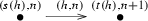
Let $Q = (I,\Omega )$ be a finite quiver, so that $s, t: \Omega \rightrightarrows I$ are the source and target maps: for $a\in \Omega$ we have .

The double of Q is a quiver $Q^{{\text {dbl}}}= (I,H = \Omega \sqcup {\overline{\Omega }})$ with the same vertex set I as for Q and the set of arrows $H = \Omega \sqcup {\overline{\Omega }}$ where $\Omega$ is the arrow set of Q and ${\overline{\Omega }}$ is a set equipped with a bijection to $\Omega$, written $\Omega \ni a \leftrightarrow a^*\in {\overline{\Omega }}$. We extend this bijection canonically to an involution on $H = \Omega \sqcup {\overline{\Omega }}$, still written $a\mapsto a^*$, and decree $s(a^*) = t(a), t(a^*)=s(a)$. For each arrow $a\in H$ we write

$$\begin{aligned} \epsilon (a) = {\left\{ \begin{array}{ll} 1 &{} \quad \text {if } a\in \Omega ,\\ -1 &{} \quad \text {if } a\in {\overline{\Omega }}.\end{array}\right. } \end{aligned}$$

Fix an integer $N\ge 1$. The graded tripled quiver $Q^{{\text {gtr}}}$ associated to Q (cf. Section 4 of [26]) is a quiver defined as follows. We give $Q^{{\text {gtr}}}$ the vertex set $I^{{\text {gtr}}} = I\times [0, N]$ where I is the vertex set of Q. If $\Omega$ is the edge set of Q and $H = \Omega \sqcup {\overline{\Omega }}$ the associated set of pairs of an edge together with an orientation, we give $Q^{{\text {gtr}}}$ the arrow set

$$\begin{aligned} \big (H\times [0, N-1]\big ) \sqcup \big (I\times [0, N-1]). \quad \text {Thus,} \end{aligned}$$

• (1) for each $h\in H$, $n\in [0, N-1]$ we have arrows (h, n) with , i.e.

  $$\begin{aligned} s(h,n) = (s(h), n) \quad \text {and} \quad t(h,n) = (t(h), n+1); \end{aligned}$$

• (2) for each $i\in I$, $n\in [0, N-1]$ we have arrows $t_{(i,n)}$ with 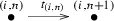, i.e.

  $$\begin{aligned} s(t_{i,n}) = (i,n) \quad \text {and} \quad t(t_{(i,n)}) = (i,n+1). \end{aligned}$$

More discussion can be found in [26, §4].

2.3 Path algebras

Let $S = \bigoplus _i k e_i$ be a commutative semisimple algebra over a field k, with orthogonal system of idempotents $\{e_i\}$. Suppose A is an algebra with homomorphism $S\rightarrow A$. We say that $x\in A$ has diagonal Peirce decomposition if $\displaystyle x\in \bigoplus _{i\in I} e_iAe_i$, or equivalently if it lies in the centralizer $Z_{A}(S)$.

Let $Q=(I,H)$ be a quiver. The path algebra kQ of Q is defined as follows: Let S denote the finite-dimensional (semisimple commutative) k-algebra $S = \bigoplus _{i\in I} ke_i$ with idempotents $e_i$ labelled by the vertices $i\in I$. We define an S-bimodule $B = B(Q)$, with k-basis labelled by the arrows, where the S-bimodule structure takes arrows to be directed “left-to-right,” so $e_iae_j =0$ unless $i = s(a), j=t(a)$, and so that $e_{s(a)}ae_{t(a)} = a$. Then the path algebra kQ is defined to be the tensor algebra $T_S(B(Q))$.

It is natural to grade the path algebra kQ of any quiver $Q = (I,H)$—for example, $kQ^{{\text {dbl}}}$— using the normal grading on a tensor algebra, thus the semisimple algebra S lies in degree 0 and the arrows $h\in H$ lie in degree 1.

If A is any S-algebra, we write A[t] for the associative S algebra obtained by adjoining a central variable t (thus every element of A commutes with t). The algebra A[t] is graded by t-degree, and hence if we take $A = kQ^{{\text {dbl}}}$, the algebra $kQ^{{\text {dbl}}}[t]$ is naturally bi-graded, but we will only use the total grading, with respect to which $\deg (t)=1$. Using the above grading for the path algebra $kQ^{{\text {gtr}}}$, we obtain a graded algebra homomorphism

$$\begin{aligned}&kQ^{{\text {dbl}}}[t]\longrightarrow kQ^{{\text {gtr}}}/J \quad \text {by taking }\\&e_i\mapsto \sum _n e_{(i,n)}+J, \;\; i\in I, \quad h\mapsto \sum _n (h,n)+J, \;\; h\in H, \quad t\mapsto \sum _{(i,n)}t_{(i,n)}+J, \end{aligned}$$

where J denotes the two-sided ideal

$$\begin{aligned} J \!=\! \Big (\big \{ t_{(s(h), n)}\cdot (h, n+1) \!-\! (h,n)\cdot t_{(t(h),n+1)}\; \big | \; h\in H, \quad n\in [0,N-2]\big \}\Big ). \end{aligned}$$

(2.1)

The graded algebra $kQ^{{\text {gtr}}}$ has the property $kQ^{{\text {gtr}}}_{\ge N+1} = 0$, so we obtain a homomorphism

$$\begin{aligned} kQ^{{\text {dbl}}}[t]_{_{[0,N]}} := kQ^{{\text {dbl}}}[t]/kQ^{{\text {dbl}}}[t]_{\ge N+1}\longrightarrow kQ^{{\text {gtr}}}/J. \end{aligned}$$

(2.2)

The above discussion thus shows:

Lemma 2.2

Let $kQ^{{\text {gtr}}}{\text {-mod}}_J$ denote the category of finite-dimensional left modules for $kQ^{{\text {gtr}}}$ annihilated by J, and furthermore let $kQ^{{\text {dbl}}}[t]_{[0,N]}{\text {-gr}}_{[0,N]}$ denote the category of finite-dimensional graded left $kQ^{{\text {dbl}}}[t]$-modules concentrated in degrees [0, N]. Then the homomorphism (2.2) determines an equivalence of categories:

$$\begin{aligned} kQ^{{\text {gtr}}}{\text {-mod}}_J \xrightarrow {\simeq } kQ^{{\text {dbl}}}[t]_{[0,N]}{\text {-gr}}_{[0,N]}. \end{aligned}$$

2.4 Universal localizations

We briefly review some aspects of universal localizations that may be unfamiliar to the reader, using Chapter 4 of [28] as our reference; see also [9].

Suppose that R is a ring with 1 and $\Sigma$ is a set of elements of R. Then there is a ring $R_\Sigma$ with a homomorphism $R\rightarrow R_\Sigma$ that is universal with respect to the property that for every $r\in \Sigma$, r becomes invertible in $R_\Sigma$, i.e. r has a two-sided inverse $r^{-1}$ in $R_\Sigma$. The ring $R_\Sigma$ is called the universal localization of R at $\Sigma$; an alternative notation that is sometimes preferable is $\Sigma ^{-1}R$. The universal localization is constructed as follows: letting $\Sigma ^{-1}$ denote the set of symbols $a^{-1}$ for $a\in \Sigma$, we define

$$\begin{aligned} \Sigma ^{-1}R = R_\Sigma := R\langle \Sigma ^{-1}\rangle /(\{a^{-1}a -1, a a^{-1}-1 \; |\; a\in \Sigma \}). \end{aligned}$$

This evidently has the universal property claimed, though very little else can be deduced about $R_\Sigma$ from this construction. Another more illuminating construction (which allows one to invert morphisms between arbitrary projective modules) is given in Theorem 4.1 of [28].

We however will only need the following properties, which follow immediately from the universal property.

Proposition 2.3

Suppose R is a ring with 1.

• (1) If $t\in Z(R)$ is central, then $R_{\{t\}}$ is isomorphic to the Øre localization of R at t.

• (2) If $\Sigma , \Sigma '\subseteq R$ are subsets, let ${\overline{\Sigma }}'$ denote the image of $\Sigma '$ in $R_\Sigma$. Then $(R_\Sigma )_{{\overline{\Sigma }}'} \cong R_{\Sigma \cup \Sigma '}$.

• (3) Given a two-sided ideal $I\subseteq R$, let ${\overline{\Sigma }}$ denote the image of $\Sigma$ in R/I and $I_\Sigma$ denote the two-sided ideal in $R_\Sigma$ generated by I. Then $(R/I)_{{\overline{\Sigma }}} \cong R_\Sigma /I_\Sigma$.

2.5 Multiplicative preprojective algebras

We review the multiplicative preprojective algebra of a quiver Q as defined in [10].

Given a quiver Q with double $Q^{{\text {dbl}}}= (I,H)$, for each arrow $a\in H$ of $Q^{{\text {dbl}}}$, we define $g_a = 1 + aa^*\in kQ^{{\text {dbl}}}$. Write $L_Q$ for the algebra obtained by universal localization of $kQ^{{\text {dbl}}}$ inverting $\Sigma = \{g_a\; |\; a\in H\}$. Identify the tuple $q\in (k^\times )^I$ with the element $\sum _{i\in I} q_i e_i\in S$. Crawley-Boevey and Shaw choose an ordering of the arrows in H and define $\displaystyle \rho _{{\text {CBS}}} = \prod \nolimits ^{\longrightarrow }_{a\in H} g_a^{\epsilon (a)} - q$ (the arrow over the product indicates that it is taken in the chosen order). It is proven in [10, §2] that, up to isomorphism, the quotient algebra $L_Q/(\rho _{{\text {CBS}}})$ does not depend on the choice of ordering. Thus, in this paper we specifically fix an ordering $\Omega = \{a_1, \dots , a_g\}$ on the arrows in Q, and let

$$\begin{aligned} \rho _{{\text {CBS}}} = g_{a_1}g_{a_2}\dots g_{a_g} g_{a_1^*}^{-1} \dots g_{a_g^*}^{-1} -q. \end{aligned}$$

(2.3)

Definition 2.4

Following [10, Definition 1.2], the associated multiplicative preprojective algebra is defined to be

$$\begin{aligned} \Lambda ^q = \Lambda ^q(Q) = L_Q/(\rho _{{\text {CBS}}}), \end{aligned}$$

where $\rho _{{\text {CBS}}}$ is defined as in (2.3).

2.6 Homogenized multiplicative preprojective algebras

A principal tool in this paper is a certain graded algebra ${{{\mathsf {A}}}}$ that “homogenizes” the multiplicative preprojective algebra $\Lambda ^q$. Here we construct the algebra ${{{\mathsf {A}}}}$ and collect some basic facts about ${{{\mathsf {A}}}}$ and its relation to the multiplicative preprojective algebra $\Lambda ^q$.

Thus, fix a quiver Q. Recall that we consider $kQ^{{\text {dbl}}}[t]$ as a nonnegatively graded algebra, with the generators $a\in H, t$ all in degree 1, and $S = \oplus _{i\in I} ke_i$ in degree 0. We let

$$\begin{aligned} G_a := t^2 + a a^* \in kQ^{{\text {dbl}}}[t] \quad \text {for all} \quad a\in H. \end{aligned}$$

Remark 2.5

Each $G_a$ has diagonal Peirce decomposition: more precisely,

$$\begin{aligned} e_{s(a)}G_a = e_{s(a)}t^2 + aa^* = G_a e_{s(a)}, \quad \text {and} \quad e_iG_a = e_it^2 = t^2 e_i = G_a e_i \quad \text {for }i\ne s(a). \end{aligned}$$

We note the obvious equalities

$$\begin{aligned} G_a a = aG_{a^*}, \quad a^* G_a = G_{a^*} a^*. \end{aligned}$$

(2.4)

Given $q \in (k^\times )^I$, we identify q with $q:= \sum _{i\in I} q_ie_i\in kQ^{{\text {dbl}}}$, a sum of idempotents in the path algebra (which thus also has diagonal Peirce decomposition).

Analogously to [10], we write ${{{\mathsf {L}}}}_t$ for the universal localization of the algebra $kQ^{{\text {dbl}}}[t]$ in which the elements $\{G_a, a\in H\}$, and t are inverted. The algebra ${{{\mathsf {L}}}}_t$ is graded and contains invertible elements $\displaystyle g_a = t^{-2}G_a = 1 + \frac{a}{t}\frac{a^*}{t}$ in graded degree 0. Moreover we have $({{{\mathsf {L}}}}_t)_0 \cong L_Q$, where as reviewed above $L_Q$ is the universal localization of $kQ^{{\text {dbl}}}\cong kQ^{{\text {dbl}}}[t^{\pm 1}]_0$ at the elements $g_a$, $a\in H$. As above, fix an ordering $\Omega = \{a_1, \dots , a_g\}$ on the arrows in Q. Write

$$\begin{aligned} D= & {} G_{a_1}\dots G_{a_g}, \quad D^* = q(G_{a_g^*}\dots G_{a_1^*}), \end{aligned}$$

(2.5)

$$\begin{aligned} \rho= & {} D - D^* = (G_{a_1}\dots G_{a_g}) - q(G_{a_g^*}\dots G_{a_1^*}) \in kQ^{{\text {dbl}}}[t]. \end{aligned}$$

(2.6)

Definition 2.6

We write ${{{\mathsf {A}}}}= kQ^{{\text {dbl}}}[t]/(\rho )$, where $(\rho )$ denotes the two-sided ideal generated by $\rho$.

The element $\rho$ has diagonal Peirce decomposition, and so $\rho e_i = e_i \rho$, and $(\rho ) = (\{\rho e_i| i\in I\})$.

Proposition 2.7

Write $\Sigma = \{G_a \; | \; a\in H\}\cup \{t\}$. We have:

• (1) ${{{\mathsf {A}}}}$ is a graded algebra where $a_i, a_i^*$ and t have degree 1 (and $S = \sum _{i\in I} ke_i$ lies in degree 0).

• (2) The universal localization

  $$\begin{aligned} \Lambda _t:= \Sigma ^{-1}{{{\mathsf {A}}}}\end{aligned}$$

  (2.7)

  of ${{{\mathsf {A}}}}$ obtained by inverting all $G_a, a\in H$, and t, is a graded algebra, and $\Lambda _t \cong \Lambda ^q(Q)[t^{\pm 1}]$ where $\Lambda ^q(Q)=: \Lambda ^q$ denotes the multiplicative preprojective algebra of [10].

Proof

This almost all follows from the above discussion. The isomorphism (2.7) of part (2) of Proposition 2.7 follows from Proposition 2.3. $\square$

3 Representations and their moduli

3.1 Representations of $kQ^{{\text {dbl}}}$ and $kQ^{{\text {gtr}}}$

Fixing some $N\ge 2g$, where g is the number of arrows in Q, we form the graded-tripled quiver $Q^{{\text {gtr}}}$ associated to Q as above.¹ Given a dimension vector $\alpha \in {\mathbb {Z}}_{\ge 0}^I$ for the quiver $Q^{{\text {dbl}}}$, we write $\alpha ^{{\text {gtr}}}\in {\mathbb {Z}}_{\ge 0}^{I\times [0,N]}$ for the dimension vector for $kQ^{{\text {gtr}}}$ for which $\alpha ^{{\text {gtr}}}_{i,n} = \alpha _i$ for all $n\in [0,N]$. We write ${\text {Rep}}(kQ^{{\text {dbl}}},\alpha )$ for the space of representations of $kQ^{{\text {dbl}}}$ with on the I-graded vector space V with $V_i = k^{\alpha _i}$ for all $i \in I$, so that V has dimension vector $\alpha$ and ${\mathbb {G}} = \prod _i GL(\alpha _i)$ for the automorphism group; thus

$$\begin{aligned} {\text {Rep}}(kQ^{{\text {dbl}}},\alpha ) := \prod _{h\in H} {\text {Hom}}(k^{\alpha _{s(h)}}, k^{\alpha _{t(h)}}). \end{aligned}$$

Similarly we write ${\text {Rep}}(kQ^{{\text {gtr}}},\alpha ^{{\text {gtr}}})$ for the space of representations of $kQ^{{\text {gtr}}}$ with dimension vector $\alpha ^{{\text {gtr}}}$, and ${\mathbb {G}}^{{\text {gtr}}}$ for the automorphism group.

As in the construction of Section 4.3 of [26], there is a natural “induction functor” from the category of representations of $kQ^{{\text {dbl}}}$ with dimension vector $\alpha$ to the category of representations of $kQ^{{\text {gtr}}}$ of dimension vector $\alpha ^{{\text {gtr}}}$. The construction proceeds as follows. To a representation V of $kQ^{{\text {dbl}}}$ we may associate the ${\mathbb {Z}}_{\ge 0}$-graded vector space V[t], and let arrows h of $Q^{{\text {dbl}}}$ act as multiplication followed by shift-of-grading. This makes V[t] into a graded left $kQ^{{\text {dbl}}}[t]$-module. We then form $V[t]/V[t]_{\ge N+1}$, a graded left $kQ^{{\text {dbl}}}[t]_{[0,N]}$-module, and finally apply Lemma 2.2 to get a representation of $kQ^{{\text {gtr}}}$: in fact, a representation of the quotient $kQ^{{\text {gtr}}}/J$ where J is as in (2.1).

More concretely, the above construction is the following. Suppose we have a representation $V = (V_i)_{i \in I}$ of $kQ^{{\text {dbl}}}$ of dimension vector $\alpha$. We obtain a representation of $kQ^{{\text {dbl}}}[t]$ on a vector space $V_{\bullet , \bullet }$ of dimension vector $\alpha ^{{\text {gtr}}}$ defined by setting $V_{\bullet ,\bullet } = V\times [0,N]$ where

• (1) the grading is given by $V_{i,n} := V_i\times \{n\}$ for all $n\in [0,N]$;

• (2) the action of the generators $t_{i,n}$ of $kQ^{{\text {gtr}}}$ for $(i,n) \in I\times [0,N-1]$ is given by $\text {id}_{V_i}\times \sigma$, where $\sigma :[0,N-1] \rightarrow [0,N]$ is given by $\sigma (n)=n+1$; and

• (3) the action of each generator $(h,n)\in H\times [0,N-1]$ is given by

  $$\begin{aligned} h\times \sigma :V_{s(h),n} \rightarrow V_{t(h),n+1} \end{aligned}$$

The construction determines a morphism of algebraic varieties (“induction”)

$$\begin{aligned}&{{\mathsf {Ind}}}^\circ : {\text {Rep}}(kQ^{{\text {dbl}}},\alpha )\longrightarrow {\text {Rep}}(kQ^{{\text {gtr}}}, \alpha ^{{\text {gtr}}}).\\&\text {Write } \quad {\mathbb {G}} = \prod _i GL(V_{i})\quad \text {and}\quad {\mathbb {G}}^{{\text {gtr}}}= \prod _{(i,n)\in I\times [a,b]} GL(V_{i,n}) \cong \prod _{n\in [a,b]}{\mathbb {G}}, \end{aligned}$$

with the diagonal homomorphism $\displaystyle {\text {diag}}: {\mathbb {G}}\rightarrow {\mathbb {G}}^{{\text {gtr}}}\cong \prod \nolimits _{n\in [a,b]} {\mathbb {G}}$. Then the morphism ${{\mathsf {Ind}}}^\circ$ is $({\mathbb {G}}, {\mathbb {G}}^{{\text {gtr}}})$-equivariant. We thus get a natural ${\mathbb {G}}^{{\text {gtr}}}$-equivariant morphism

$$\begin{aligned} {{\mathsf {Ind}}}: {\mathbb {G}}^{{\text {gtr}}}\times _{{\mathbb {G}}} {\text {Rep}}(kQ^{{\text {dbl}}},\alpha )\longrightarrow {\text {Rep}}(kQ^{{\text {gtr}}}, \alpha ^{{\text {gtr}}}). \end{aligned}$$

(3.1)

Thus, given a representation $(a_h: V_{s(h)}\rightarrow V_{t(h)})_{h \in H}$ of $kQ^{{\text {dbl}}}$ on V, and $(g_{i,n})\in {\mathbb {G}}^{{\text {gtr}}}$, we have

$$\begin{aligned} {{\mathsf {Ind}}}\big ((g_{i,n}), a_h\big ) = \big ((h,n), t_{i,n}\big ) \, \text {where} \, (h,n) = g_{t(h),n+1}a_h g_{s(h),n}^{-1}\, \text {and} \, t_{i,n} = g_{i,n+1} g_{i,n}^{-1}. \end{aligned}$$

Proposition 3.1

The map ${{\mathsf {Ind}}}$ of (3.1) defines a ${\mathbb {G}}^{{\text {gtr}}}$-equivariant open immersion of ${\mathbb {G}}^{{\text {gtr}}}\times _{{\mathbb {G}}} {\text {Rep}}(kQ^{{\text {dbl}}},\alpha )$ in ${\text {Rep}}(kQ^{{\text {gtr}}}/J,\alpha ^{{\text {gtr}}})$, whose image consists of those $\big ((h,n), t_{i,n}\big )$ for which:

$$\begin{aligned} t_{i,n}\text { is an isomorphism for all }n\in [0,N-1].\qquad (\dagger ) \end{aligned}$$

Proof

This follows from the discussion above, indeed one can readily adapt the proof of the corresponding statment for Nakajima quiver varieties, see [26, Proposition 4.1]. $\square$

3.2 Representations of ${{{\mathsf {A}}}}$ and ${{{\mathsf {A}}}}_{[0,N]}$

Let ${{{\mathsf {A}}}}{\text {-Gr}}$ denote the category of graded left ${{{\mathsf {A}}}}$-modules. We also consider the category ${{{\mathsf {A}}}}_{[0,N]}{\text {-Gr}}_{\ge 0}$ of those graded left ${{{\mathsf {A}}}}_{[0,N]}$-modules M for which $M_i=0$ for $i\notin [0,N]$. We remark that ${{{\mathsf {A}}}}_{[0,N]}{\text {-Gr}}_{\ge 0}$ can naturally be viewed as a full subcategory of the category ${{{\mathsf {A}}}}_{[0,N]}{\text {-Gr}}$ of all graded left ${{{\mathsf {A}}}}_{[0,N]}$-modules, hence also of ${{{\mathsf {A}}}}{\text {-Gr}}$. Define a functor of truncation,

$$\begin{aligned} \tau _{[0,N]}: {{{\mathsf {A}}}}{\text {-Gr}} \longrightarrow {{{\mathsf {A}}}}_{[0,N]}{\text {-Gr}}_{\ge 0}, \end{aligned}$$

by $M\mapsto \tau _{[0,N]}M := M_{\ge 0}/M_{\ge N+1}$. As above, we have a graded vector space injection $\tau _{[0,N]}(M)\rightarrow M$ that is the identity on the mth graded piece for $m\in [0,N]$ and is zero elsewhere; this map is ${{{\mathsf {A}}}}_{\le m}$-linear on $M_{N-m}$.

3.3 Representations of ${{{\mathsf {A}}}}$ and $\Lambda ^q$

We note:

Remark 3.2

The functor $\Lambda _t{\text {-Gr}}\longrightarrow \Lambda ^q{\text {-Mod}}$, $M\mapsto M_0$, is an equivalence of categories.

Recall from (2.7) that, letting $\Sigma = \{G_a \; | \; a\in H\}\cup \{t\}$, we have a graded algebra isomorphism $\Sigma ^{-1}{{{\mathsf {A}}}}\cong \Lambda _t = \Lambda ^q[t^{\pm 1}]$, and hence a graded algebra homomorphism ${{{\mathsf {A}}}}\rightarrow \Lambda ^q[t^{\pm 1}]$. Given a left or right $\Lambda ^q$-module $\overline{{\mathcal {M}}}$, we form a graded left or right $\Lambda _t$-module ${\mathcal {M}} = \overline{{\mathcal {M}}}[t^{\pm 1}]$, and thus a graded ${{{\mathsf {A}}}}$-module $M = {\mathcal {M}}[t]={\mathcal {M}}[t^{\pm 1}]_{\ge 0}$. This defines a functor

$$\begin{aligned} R: \Lambda ^q{\text {-Mod}}\longrightarrow {{{\mathsf {A}}}}{\text {-Gr}}_{\ge 0}. \end{aligned}$$

In the opposite direction, we have a functor $(\Lambda _t\otimes _{{{{\mathsf {A}}}}} -)_0: {{{\mathsf {A}}}}{\text {-Gr}}_{\ge 0}\rightarrow \Lambda ^q{\text {-Mod}}$. We have:

Lemma 3.3

• (1) The functors form an adjoint pair.

• (2) If $\overline{{\mathcal {M}}}$ is a finite-dimensional left $\Lambda ^q$-module then the graded left ${{{\mathsf {A}}}}$-module $M = \overline{{\mathcal {M}}}[t]$ is finitely generated and projective as a left $S_t$-module and as a left k[t]-module. Moreover, we have ${\text {Hom}}_{k[t]}(M,k[t]) \cong {\text {Hom}}_k(\overline{{\mathcal {M}}},k)[t]$ as a graded right ${{{\mathsf {A}}}}$-module.

Proof

The first statement follows from the isomorphism $\Lambda _t \cong \Lambda ^q[t^{\pm 1}]$ along with the equivalence of categories noted in the above remark. Indeed

$$\begin{aligned} \begin{aligned} \mathrm {Hom}(M,N[t])&\cong \mathrm {Hom}(M,N[t^{\pm 1}]) \cong \mathrm {Hom}(\Lambda _t\otimes _A M,N[t^{\pm 1}]) \\&\cong \mathrm {Hom}((\Lambda _t\otimes _A M)_0,N), \end{aligned} \end{aligned}$$

where the second isomorphism follow from universality. The second statement follows immediately from the definitions. $\square$

3.4 Representation spaces and group actions

Because the multiplicative preprojective algebra $\Lambda ^q$ is the quotient $L_Q/(\rho _{{\text {CBS}}})$ of the localization $L_Q$ of $kQ^{{\text {dbl}}}$ by the ideal generated by $\rho _{{\text {CBS}}}$, the space ${\text {Rep}}(\Lambda ^q,\alpha )$ of left $\Lambda ^q$-modules with dimension vector $\alpha$ is naturally a locally closed subscheme of ${\text {Rep}}(kQ^{{\text {dbl}}},\alpha )$: it is the closed subset, defined by vanishing of $\rho _{{\text {CBS}}}$, of the open set defined by invertibility of the elements $g_a$.

Similarly, the algebra ${{{\mathsf {A}}}}_{[0,N]}$ is a quotient of $kQ^{{\text {dbl}}}[t]_{[0,N]}$ and thus, via Lemma 2.2, the space ${\text {Rep}}_{{\text {gr}}}({{{\mathsf {A}}}}_{[0,N]}, \alpha ^{{\text {gtr}}})$ of graded left ${{{\mathsf {A}}}}_{[0,N]}$-modules concentrated in degrees [0, N] is identified with a closed subscheme of ${\text {Rep}}(kQ^{{\text {gtr}}}, \alpha ^{{\text {gtr}}})$ defined by the vanishing of the images of $\rho$ and J in $kQ^{{\text {gtr}}}$.

It is immediate from the construction of Sect. 3.1 that:

Proposition 3.4

(cf. Prop. 4.7 of [26]) The morphism ${{\mathsf {Ind}}}$ of (3.1) restricts to an open immersion:

$$\begin{aligned} {{\mathsf {Ind}}}: {\mathbb {G}}^{{\text {gtr}}}\times _{{\mathbb {G}}} {\text {Rep}}(\Lambda ^q,\alpha ) \rightarrow {\text {Rep}}_{{\text {gr}}}({{{\mathsf {A}}}}_{[0,N]}, \alpha ^{{\text {gtr}}}). \end{aligned}$$

Its image consists of those representations on which the elements $t, G_a$ act invertibly whenever their domain and target lie in the range [0, N].

Corollary 3.5

The map ${{\mathsf {Ind}}}$ defines an open immersion of moduli stacks

$$\begin{aligned} {\text {Rep}}(\Lambda ^q,\alpha )/{\mathbb {G}}\rightarrow {\text {Rep}}_{{\text {gr}}}({{{\mathsf {A}}}}_{[0,N]}, \alpha ^{{\text {gtr}}})/{\mathbb {G}}^{{\text {gtr}}}. \end{aligned}$$

3.5 Semistability and stability

We next discuss (semi)stability of representations and the corresponding GIT quotients.

For any quiver $Q = (I,\Omega )$ with dimension vector $\alpha \in {\mathbb {Z}}^I_{\ge 0}$, a GIT stability condition is given by $\theta \in {\mathbb {Z}}^I_{\ge 0}$ satisfying $\sum _i \theta _i\alpha _i = 0$. The vector $\theta$ determines a character $\chi _{\theta }: \prod _i GL(\alpha _i)\rightarrow {{\mathbb {G}}}_m$, $\chi (g_i)_{i\in I} = \prod _i \det (g_i)^{\theta _i}$, and the condition $\sum _i \theta _i\alpha _i = 0$ guarantees that the diagonal copy $\Delta ({{\mathbb {G}}}_m)$ of ${{\mathbb {G}}}_m$ in $\prod _i GL(\alpha _i)$ lies in the kernel of $\chi$; we require this because $\Delta ({{\mathbb {G}}}_m)$ acts trivially on ${\text {Rep}}(Q,\alpha )$. Given dimension vectors $\beta ,\alpha$, we write $\beta <\alpha$ if $\beta \ne \alpha$ and $\beta _i\le \alpha _i$ for all $i\in I$.

We now turn to stability conditions for the doubled and tripled quivers $Q^{{\text {dbl}}}$ and $Q^{{\text {gtr}}}$ for a fixed quiver Q. Suppose $\theta$ is a stability condition for $Q^{{\text {dbl}}}$ and dimension vector $\alpha$. We construct a stability condition $\theta ^{{\text {gtr}}}$ for $Q^{{\text {gtr}}}$ with dimension vector $\alpha ^{{\text {gtr}}}$ as follows. For a representation M of $kQ^{{\text {gtr}}}$ of dimension vector $\alpha ^{{\text {gtr}}}$, we write $\delta _{i,n}(M) := \dim (M_{i,n})$; we will write $\theta ^{{\text {gtr}}}$ as a linear combination of the $\delta _{i,n}$. Also, we note that it suffices to construct a rational linear functional $\theta ^{{\text {gtr}}}$, since any positive integer multiple of $\theta ^{{\text {gtr}}}$ evidently defines the same stable and semistable loci. We fix an ordering on the vertices of Q, identifying $I = \{1, \dots , r\}$. and a positive integer $\displaystyle T \gg 0.$ We define:

$$\begin{aligned} \theta ^{{\text {gtr}}}:= \sum _{i=1}^r T^i\big [\delta _{i,N}-\delta _{i,0}\big ] + \sum _{i\in I} \theta _i \delta _{i,0}. \end{aligned}$$

Proposition 3.6

Suppose $M = {{\mathsf {Ind}}}(N)$ for some representation N of $kQ^{{\text {dbl}}}$ with dimension vector $\alpha$. Then M is semistable, respectively stable, with respect to $\theta ^{{\text {gtr}}}$ if and only if N is semistable, respectively stable, with respect to $\theta$.

The proof is an easy adaptation of that of Proposition 4.12(4) of [26].

We remark that the above construction does not match [26]: there we chose to construct a stability $\theta ^{{\text {gtr}}}$ for $Q^{{\text {gtr}}}$ that would be nondegenerate if $\theta$ was, whereas here we ignore this possible requirement. While it would be possible to copy the construction of a stability $\theta ^{{\text {gtr}}}$ from [26] and prove analogues of the statements of [26], there are cases important to multiplicative quiver varieties in which it is not possible to find a stability condition for $kQ^{{\text {dbl}}}$ that is nondegenerate in the sense used in [26]: for example, the case when Q has a single vertex and loops based at that vertex, with dimension vector $\alpha = n>1$. However, again for multiplicative quiver varieties, in some interesting cases the choice of the parameter q can guarantee that every semistable representation of $\Lambda ^q$ is automatically stable (though not for numerical reasons, as nondegeneracy guarantees). Indeed, we say $q = (q_i)_{i\in I}\in (k^\times )^I$ is a primitive $\alpha$th root of unity if $q^\alpha :=\prod q_i^{\alpha _i} = 1$ and $q^\beta \ne 1$ for all $0<\beta <\alpha$. We have:

Lemma 3.7

([10], Lemma 1.5)

• (1) Suppose that M is a representation of $\Lambda ^q$ with dimension vector $\alpha$. Then $q^\alpha = 1$.

• (2) In particular, if q is a primitive $\alpha$th root of 1, then every representation of $\Lambda ^q$ of dimension vector $\alpha$ is $\theta$-stable for every $\theta$.

For example, if $Q= (\{*\},E)$ where E has g loops at $*$, $\alpha = n$, and q is a primitive nth root of 1, then every representation of $\Lambda ^q$ of dimension n is stable for every $\theta$; the corresponding moduli space of representations of $\Lambda ^q$ is the character variety ${\text {Char}}(\Sigma _g, GL_n, q{\text {Id}})$ of the introduction.

Remark 3.8

It would be interesting to characterize those stability conditions $\theta ^{{\text {gtr}}}$ for $kQ^{{\text {gtr}}}$ with the property that there is a stability condition $\theta$ for $kQ^{{\text {dbl}}}$ so that if $M = {{\mathsf {Ind}}}(N)$ then M is $\theta ^{{\text {gtr}}}$-(semi)stable if and only if N is $\theta$-(semi)stable.

Notation 3.9

We write

$$\begin{aligned} {\mathcal {M}}_{\theta }^q(\alpha ) := {\text {Rep}}(\Lambda ^q,\alpha )//_{\theta }{\mathbb {G}} \;\;\text {and}\;\; {\mathcal {M}}_{\theta }^q(\alpha )^{{\text {s}}} := {\text {Rep}}(\Lambda ^q,\alpha )^{\theta -{\text {s}}}//_{\theta }{\mathbb {G}} \end{aligned}$$

for the coarse moduli spaces determined by a stability condition $\theta$.

3.6 Moduli stacks and resolutions

The moduli stacks

$$\begin{aligned} {\text {Rep}}(\Lambda ^q,\alpha )^{\theta {\text {-ss}}}/{\mathbb {G}}\hbox { and } {\text {Rep}}_{{\text {gr}}}({{{\mathsf {A}}}}_{[0,N]}, \alpha ^{{\text {gtr}}})^{\theta ^{{\text {gtr}}}{\text {-ss}}}/{\mathbb {G}}^{{\text {gtr}}}\end{aligned}$$

are never Deligne–Mumford stacks: the diagonal copy of ${{\mathbb {G}}}_m$ in ${\mathbb {G}}$, respectively ${\mathbb {G}}^{{\text {gtr}}}$, always acts trivially on ${\text {Rep}}(\Lambda ^q,\alpha )$, respectively ${\text {Rep}}_{{\text {gr}}}({{{\mathsf {A}}}}_{[0,N]}, \alpha ^{{\text {gtr}}})^{\theta ^{{\text {gtr}}}{\text {-ss}}}$. Thus, the moduli stack of stable representations ${\text {Rep}}(\Lambda ^q,\alpha )^{\theta {\text {-s}}}/{\mathbb {G}}$ is always a ${{\mathbb {G}}}_m$-gerbe over the moduli space ${\mathcal {M}}_{\theta }^q(\alpha )^{{\text {s}}}$ of stable representations.

However, one can make a choice of subgroup ${\mathbb {S}}\subset {\mathbb {G}}$ that ensures that the quotient stack ${\text {Rep}}(\Lambda ^q,\alpha )^{\theta -{\text {s}}}/{\mathbb {S}}$ is a Deligne–Mumford stack and that ${\text {Rep}}(\Lambda ^q,\alpha )^{\theta -{\text {s}}}/{\mathbb {S}}\rightarrow {\mathcal {M}}_{\theta }^q(\alpha )^{{\text {s}}}$ is a finite gerbe (indeed a principal BH-bundle for a finite abelian group H). Indeed, for example, we can choose any character $\rho : {\mathbb {G}}^{{\text {gtr}}}\rightarrow {{\mathbb {G}}}_m$ for which the composite with the diagonal embedding $\rho \circ \Delta : {{\mathbb {G}}}_m\rightarrow {{\mathbb {G}}}_m$ is nontrivial, hence surjective. Then ${\mathbb {S}}^{{\text {gtr}}}:=\ker (\rho )$ has the property that ${\mathbb {G}}^{{\text {gtr}}}= {\mathbb {S}}^{{\text {gtr}}}\cdot \Delta ({{\mathbb {G}}}_m)$ and similarly letting ${\mathbb {S}}= {\mathbb {G}}\cap {\mathbb {S}}^{{\text {gtr}}}$ we have ${\mathbb {G}} = {\mathbb {S}}\cdot \Delta ({{\mathbb {G}}}_m)$. Moreover, since $\Delta ({{\mathbb {G}}}_m)$ is the stabilizer of every point of ${\text {Rep}}(\Lambda ^q,\alpha )^{\theta {\text {-s}}}$ and $H := \Delta ({{\mathbb {G}}}_m)\cap {\mathbb {S}}$ is finite, we get:

Lemma 3.10

The quotient ${\text {Rep}}(\Lambda ^q,\alpha )^{\theta {\text {-s}}}/{\mathbb {S}}$ is a Deligne–Mumford stack and the natural morphism

$$\begin{aligned} {\text {Rep}}(\Lambda ^q,\alpha )^{\theta {\text {-s}}}/{\mathbb {S}}\rightarrow {\mathcal {M}}_{\theta }^q(\alpha )^{{\text {s}}} \end{aligned}$$

is a torsor for the commutative group stack BH (in particular, is a finite gerbe over ${\mathcal {M}}_{\theta }^q(\alpha )^{{\text {s}}}$).

By construction, we have an open immersion:

$$\begin{aligned} {\text {Rep}}(\Lambda ^q,\alpha )^{\theta {\text {-s}}}/{\mathbb {S}}\hookrightarrow {\text {Rep}}_{{\text {gr}}}({{{\mathsf {A}}}}_{[0,N]}, \alpha ^{{\text {gtr}}})^{\theta ^{{\text {gtr}}}{\text {-ss}}}/{\mathbb {S}}^{{\text {gtr}}}, \end{aligned}$$

and the coarse space of the target ${\text {Rep}}_{{\text {gr}}}({{{\mathsf {A}}}}_{[0,N]}, \alpha ^{{\text {gtr}}})^{\theta ^{{\text {gtr}}}{\text {-ss}}}/{\mathbb {S}}^{{\text {gtr}}}$ is the projective moduli scheme ${\text {Rep}}_{{\text {gr}}}({{{\mathsf {A}}}}_{[0,N]}, \alpha ^{{\text {gtr}}})//_{\theta ^{{\text {gtr}}}}{\mathbb {G}}^{{\text {gtr}}}$: it is a closed subscheme of ${\text {Rep}}(kQ^{{\text {gtr}}},\alpha ^{{\text {gtr}}})//_{\theta ^{{\text {gtr}}}}{\mathbb {G}}^{{\text {gtr}}}$, which (as in [26]) is projective because $kQ^{{\text {gtr}}}$ has no oriented cycles, and hence is itself projective.

As in [26], our goal is to compactify ${\text {Rep}}(\Lambda ^q,\alpha )^{\theta {\text {-s}}}/{\mathbb {S}}$ appropriately. We therefore replace the quotient stack ${\text {Rep}}_{{\text {gr}}}({{{\mathsf {A}}}}_{[0,N]}, \alpha ^{{\text {gtr}}})^{\theta ^{{\text {gtr}}}{\text {-ss}}}/{\mathbb {S}}^{{\text {gtr}}}$ by its closed substack defined as the closure of ${\text {Rep}}(\Lambda ^q,\alpha )^{\theta {\text {-s}}}/{\mathbb {S}}$:

Notation 3.11

We denote the closure of ${\text {Rep}}(\Lambda ^q,\alpha )^{\theta {\text {-s}}}/{\mathbb {S}}$ in ${\text {Rep}}_{{\text {gr}}}({{{\mathsf {A}}}}_{[0,N]}, \alpha ^{{\text {gtr}}})^{\theta ^{{\text {gtr}}}{\text {-ss}}}/{\mathbb {S}}^{{\text {gtr}}}$ by $\overline{{\mathcal {M}}}_{{\text {st}}}$.

Lemma 3.12

The stack ${\text {Rep}}(\Lambda ^q,\alpha )^{\theta {\text {-s}}}/{\mathbb {S}}$ is smooth. The stack $\overline{{\mathcal {M}}}_{{\text {st}}}$ is integral and its coarse moduli space is a projective scheme. The natural morphism ${\text {Rep}}(\Lambda ^q,\alpha )^{\theta {\text {-s}}}/{\mathbb {S}}\hookrightarrow \overline{{\mathcal {M}}}_{{\text {st}}}$ is an open immersion.

Proof

The smoothness of ${\text {Rep}}(\Lambda ^q,\alpha )^{\theta {\text {-s}}}/{\mathbb {S}}$ is Theorem 1.10 of [10]. The remaining assertions are immediate. $\square$

We may apply the results of [22] or [14] to ${\text {Rep}}(kQ^{{\text {gtr}}}, \alpha ^{{\text {gtr}}})^{\theta ^{{\text {gtr}}}{\text {-ss}}}/{\mathbb {S}}^{{\text {gtr}}}$ and its closed substack $\overline{{\mathcal {M}}}_{{\text {st}}}$ to obtain a projective Deligne–Mumford stack (i.e., a Deligne–Mumford stack whose coarse space is a projective scheme) $\overline{{\mathcal {M}}}_{{\text {st}}}'$ equipped with a projective morphism $\overline{{\mathcal {M}}}_{{\text {st}}}'\rightarrow \overline{{\mathcal {M}}}_{{\text {st}}}$ that is an isomorphism over ${\text {Rep}}(\Lambda ^q,\alpha )^{\theta {\text {-s}}}/{\mathbb {S}}$. The stack $\overline{{\mathcal {M}}}_{{\text {st}}}'$ is itself, by construction, a global quotient of a quasiprojective variety by ${\mathbb {S}}$, and thus we may apply equivariant resolution to resolve the singularities of $\overline{{\mathcal {M}}}_{{\text {st}}}'$, to obtain:

Proposition 3.13

The smooth Deligne–Mumford stack ${\text {Rep}}(\Lambda ^q,\alpha )^{\theta {\text {-s}}}/{\mathbb {S}}$ admits an open immersion

$$\begin{aligned} {\text {Rep}}(\Lambda ^q,\alpha )^{\theta {\text {-s}}}/{\mathbb {S}}\hookrightarrow \overline{{\text {Rep}}(\Lambda ^q,\alpha )^{\theta {\text {-s}}}/{\mathbb {S}}} \end{aligned}$$

in a smooth projective Deligne–Mumford stack which is equipped with a projective morphism

$$\begin{aligned} \overline{{\text {Rep}}(\Lambda ^q,\alpha )^{\theta {\text {-s}}}/{\mathbb {S}}} \rightarrow \overline{{\mathcal {M}}}_{{\text {st}}} \end{aligned}$$

that extends the open immersion ${\text {Rep}}(\Lambda ^q,\alpha )^{\theta {\text {-s}}}/{\mathbb {S}}\hookrightarrow \overline{{\mathcal {M}}}_{{\text {st}}}$.

4 The diagonal of the algebra ${{{\mathsf {A}}}}$

4.1 Bimodule of derivations

Recall that we have fixed an ordering $\Omega = \{a_1, \dots , a_g\}$ on the arrows in Q. For $j=1, \dots , g$ we write

$$\begin{aligned} L_{a_j}= & {} G_{a_1}\dots G_{a_{j-1}}, \quad R_{a_j} = G_{a_{j+1}}\dots G_{a_g}, \quad \text {so}\quad D = L_{a_j}G_{a_j}R_{a_j},\\ L_{a_j^*}= & {} G_{a_g^*}\dots G_{a_{j+1}^*}, \quad R_{a_j^*} = G_{a_{j-1}^*}\dots G_{a_1^*}, \quad \text {so}\quad D^* = qL_{a_j^*}G_{a_j^*}R_{a_j^*}. \end{aligned}$$

Let B denote the sub-(S[t], S[t])-bimodule of $kQ^{{\text {dbl}}}[t]$ spanned by the arrows, so that $kQ^{{\text {dbl}}}[t]$ is identified with the tensor algebra $T_{S[t]}(B)$. As in [10, p. 190], the bimodule that is the target of the universal ${{{\mathsf {S}}}}$-linear bimodule derivation of $kQ^{{\text {dbl}}}[t]$ satisfies

$$\begin{aligned} \Omega _{S[t]}(kQ^{{\text {dbl}}}[t]) \cong kQ^{{\text {dbl}}}[t]\otimes _{S[t]} B\otimes _{S[t]} kQ^{{\text {dbl}}}[t], \end{aligned}$$

under which the universal derivation $\delta _{kQ^{{\text {dbl}}}[t]/S[t]}: kQ^{{\text {dbl}}}[t] \rightarrow \Omega _{S[t]}(kQ^{{\text {dbl}}}[t])$ is identified with $a \mapsto 1\otimes a\otimes 1$. As in [10, p. 190], for the universal localization ${{{\mathsf {L}}}}_t$ we also get $\Omega _{S[t]}({{{\mathsf {L}}}}_t) \cong {{{\mathsf {L}}}}_t \otimes _{kQ^{{\text {dbl}}}[t]} \Omega _{S[t]}(kQ^{{\text {dbl}}}[t]) \otimes _{kQ^{{\text {dbl}}}[t]} {{{\mathsf {L}}}}_t$ with the obvious identification of the universal derivation $\delta _{{{{\mathsf {L}}}}_t/S[t]}$. We write:

$$\begin{aligned} P_1 = {{{\mathsf {A}}}}\otimes _{S[t]} B\otimes _{S[t]} {{{\mathsf {A}}}}\cong {{{\mathsf {A}}}}\underset{kQ^{{\text {dbl}}}[t]}{\otimes } \Omega _{S[t]}(kQ^{{\text {dbl}}}[t]) \underset{kQ^{{\text {dbl}}}[t]}{\otimes } {{{\mathsf {A}}}}. \end{aligned}$$

(4.1)

The module $P_1$ is evidently projective as a bimodule. Via the above description, we obtain a collection of bimodule basis elements

$$\begin{aligned} \eta _a, a\in H, \;\;\; \text {via} \;\;\; \eta _a = 1\otimes a \otimes 1 \in {{{\mathsf {A}}}}\otimes _{S[t]} B\otimes _{S[t]} {{{\mathsf {A}}}}= P_1. \end{aligned}$$

4.2 An exact sequence

We write

$$\begin{aligned} P_0 = {{{\mathsf {A}}}}\otimes _{S[t]} {{{\mathsf {A}}}}. \end{aligned}$$

Write $\eta _i = e_i\otimes 1 = 1\otimes e_i$, $i\in I$, for the obvious bimodule generators of $P_0$. Define graded bimodule maps

$$\begin{aligned} P_0(-2g) \xrightarrow {\alpha } P_1(-1) \xrightarrow {\beta } P_0 \end{aligned}$$

(4.2)

by $\beta (\eta _a) = a \eta _{s(a)} - \eta _{t(a)} a$ for arrows a of $Q^{{\text {gtr}}}$, and

$$\begin{aligned} \alpha (\eta _i) = \sum _{a\in \Omega , s(a) = i} L_a \Delta _a R_a - \sum _{a\in \Omega , t(a)=i} qL_{a^*}\Delta _{a^*}R_{a^*}, \end{aligned}$$

(4.3)

where $\Delta _a = \delta (G_a)$ (where $\delta$ denotes the universal derivation). It is then immediate that $\alpha (\eta _i) = e_i\cdot \delta (\rho )$; in particular, letting $\theta : P_0\rightarrow (\rho )/(\rho ^2)$ denote the map defined by $\theta (p\otimes q) = p\rho q$ and writing $\phi$ for the isomorphism defined by (4.1), we have:

$$\begin{aligned} \phi \circ \alpha = \delta \circ \theta . \end{aligned}$$

(4.4)

Imitating the proof of Lemma 3.1 of [10] gives:

Lemma 4.1

The sequence

$$\begin{aligned} P_0(-2g)\xrightarrow {\alpha } P_1(-1) \xrightarrow {\beta } P_0 \xrightarrow {\gamma } {{{\mathsf {A}}}}\rightarrow 0, \end{aligned}$$

(4.5)

where $\gamma (p\otimes q) = pq$, is an exact sequence of ${\mathbb {Z}}$-graded bimodules.

Proof

As in [28, Theorem 10.3], one gets an exact sequence

$$\begin{aligned} (\rho )/(\rho ^2) \xrightarrow {\delta } \Omega _{S[t]}\big (kQ^{{\text {dbl}}}[t]\big ) \rightarrow \Omega _{S[t]} {{{\mathsf {A}}}}\rightarrow 0. \end{aligned}$$

As in [10], splicing this sequence and the defining sequence for $\Omega _{S[t]}\big ({{{\mathsf {A}}}}\big )$ and applying (4.4) gives a commutative diagram

The vertical arrows $\phi , \psi$ are isomorphisms and $\theta$ is surjective, yielding the assertion. $\square$

4.3 Dual of the map $P_0(-2g)\xrightarrow {\alpha } P_1(-1)$

Recall that the enveloping algebra of ${{{\mathsf {A}}}}$ over k[t] is

$$\begin{aligned} {{{\mathsf {A}}}}^e := {{{\mathsf {A}}}}\otimes _{k[t]}{{{\mathsf {A}}}}^{{\text {op}}}. \end{aligned}$$

We consider ${{{\mathsf {A}}}}^e$ as a left ${{{\mathsf {A}}}}^e$-module where $a\otimes a'\in {{{\mathsf {A}}}}^e$ acts by

$$\begin{aligned} a\otimes a'\cdot (x\otimes x') = ax\otimes x'a'. \end{aligned}$$

We remark that ${{{\mathsf {A}}}}^e$ naturally also has a right ${{{\mathsf {A}}}}^e$-module structure commuting with the left ${{{\mathsf {A}}}}^e$-action, where $a\otimes a'\in {{{\mathsf {A}}}}^e$ acts on the right by

$$\begin{aligned} (x\otimes x')\cdot a\otimes a' = xa\otimes a'x'. \end{aligned}$$

Given a finitely generated left ${{{\mathsf {A}}}}^e$-module, we form $P^\vee = {\text {Hom}}_{{{{\mathsf {A}}}}^e}(P, {{{\mathsf {A}}}}^e)$, the dual over the enveloping algebra; by the above discussion, this module has a right ${{{\mathsf {A}}}}^e$-module structure, which we can identify with a left ${{{\mathsf {A}}}}^e$-module structure via the isomorphism

$$\begin{aligned} ({{{\mathsf {A}}}}^e)^{{\text {op}}} \rightarrow {{{\mathsf {A}}}}^e, \quad a\otimes a' \mapsto a' \otimes a. \end{aligned}$$

We now want to calculate the dual $\alpha ^\vee$ of the map $\alpha$ of (4.2) using the formula (4.3). Note that

$$\begin{aligned} \Delta (G_a) = a\delta (a^*) + \delta (a)a^* = a \eta _{a^*} + \eta _a a^*. \end{aligned}$$

We thus find from Formula (4.3) that the $\eta _a$-component of $\alpha$ is given by

$$\begin{aligned} \alpha (\eta _i)_{\eta _a} = {\left\{ \begin{array}{ll} L_a \eta _a a^* R_a - qL_{a^*}a^*\eta _a R_{a^*} &{} \quad \text {if } a\in \Omega , i=s(a),\\ L_{a^*} a^* \eta _a R_{a^*} - qL_a \eta _a a^* R_a &{} \quad \text {if } a\in {\overline{\Omega }}, i=t(a) \end{array}\right. } \end{aligned}$$

and zero otherwise. Let $\{\eta _a^\vee \}$ denote the basis of $P_1^\vee$ dual to the basis $\{\eta _a\}$ of $P_1$; we note that

$$\begin{aligned} \eta ^\vee _a \in e_{t(a)}P_1^\vee e_{s(a)}. \end{aligned}$$

(4.6)

The above formulas then imply:

$$\begin{aligned} \alpha ^\vee (\eta _a^\vee ) = {\left\{ \begin{array}{ll} a^*R_a \eta _{s(a)}^\vee L_a - qR_{a^*} \eta _{t(a)}^\vee L_{a^*}a^* &{}\quad \text {if }a\in \Omega ,\\ R_a^*\eta _{t(a)}^\vee L_{a^*}a^* - qa^*R_a \eta _{s(a)}^\vee L_a &{}\quad \text {if }a\in {\overline{\Omega }}. \end{array}\right. } \end{aligned}$$

(4.7)

Lemma 4.2

For all $a\in \Omega$, we have

$$\begin{aligned} \alpha ^\vee \big (\eta ^\vee _a a- a^*\eta _{a^*}^\vee \big )&= G_{a^*}\big (qR_{a^*}\eta ^\vee _{t(a)} L_{a^*}\big ) - \big (qR_{a^*}\eta ^\vee _{t(a)}L_{a^*}\big )G_{a^*},\end{aligned}$$

(4.8)

$$\begin{aligned} \alpha ^\vee \big (a\eta _a^\vee - \eta _{a^*}^\vee a^*\big )&= G_a\big (R_a\eta _{s(a)}^\vee L_a\big ) - \big (R_a\eta _{s(a)}^\vee L_a\big ) G_a. \end{aligned}$$

(4.9)

Proof

These formulas follow by direct calculation using 4.7. $\square$

Lemma 4.3

If $a\in H$, $s(a)\ne i$, then $G_a D\eta ^\vee _i = D\eta _i^\vee G_a$ in $P_0^\vee$.

Proof

The element D is a product of elements of diagonal Peirce type, hence itself is of diagonal Peirce type. Thus, using $e_{s(a)}\eta _i^\vee = 0 = \eta _i^\vee e_{s(a)}$, we get

$$\begin{aligned} G_a D\eta ^\vee _i= & {} \big (G_ae_{s(a)} + (1-e_{s(a)})t^2\big )D\eta ^\vee _i = (1-e_{s(a)}t^2)D\eta ^\vee _i \\= & {} D\eta ^\vee _i(1-e_{s(a)}t^2) = D\eta ^\vee _i\big (e_{s(a)}G_a + (1-e_{s(a)})t^2\big ) = D\eta ^\vee _i G_a. \end{aligned}$$

This completes the proof. $\square$

Suppose now that ${\mathcal {M}}$ is a graded right $\Lambda _t$-module; then $M = {\mathcal {M}}_{\ge 0}$ is a graded right ${{{\mathsf {A}}}}$-submodule of ${\mathcal {M}}$. For example, we could take ${\mathcal {M}} = \Lambda _t$ itself, as in (2.7). We consider the map

$$\begin{aligned} M\otimes _{{{{\mathsf {A}}}}} P_1^\vee (1) \xrightarrow {1_{M}\otimes \alpha ^\vee } M\otimes _{{{{\mathsf {A}}}}} P_0^\vee (2g). \end{aligned}$$

Remark 4.4

We note that, under the above hypothesis on M, for any product Q of elements $G_a$, $a\in H$, of degree $\deg (Q)$, the elements $Qt^{-\deg (Q)}$ and $t^{\deg (Q)}Q^{-1}$ of $\Lambda _t$ give well defined operators of right multiplication on M that satisfy all relations in $\Lambda _t$.

Proposition 4.5

Suppose that $M = {\mathcal {M}}_{\ge 0}$ for a graded right $\Lambda _t$-module ${\mathcal {M}}$. Then for all $m\in M$ and all $i\in I$ and $1\le j \le g$,

• (1) the elements $m\big (G_{a_j} D \eta ^\vee _i - D\eta _i^\vee G_{a_j}\big )$, $m\big (G_{a_j^*} D \eta ^\vee _i - D\eta _i^\vee G_{a_j^*}\big )$, and

• (2) the elements $m\big (a_j^* Dt^{-2}\eta _{s(a_j)}^\vee - Dt^{-2}\eta _{t(a_j)}^\vee a_j^*\big )$, $m\big (a_j Dt^{-2}\eta _{t(a_j)}^\vee - Dt^{-2}\eta _{s(a_j)}^\vee a_j\big )$

lie in ${\text {Im}}(1_{\Lambda _t}\otimes \alpha ^\vee ) \subseteq M\otimes _{{{{\mathsf {A}}}}} P_0^\vee (2g)$.

Proof

(1) We first prove that $m\big (G_{a_j} D \eta ^\vee _i - D\eta _i^\vee G_{a_j}\big ) \in {\text {Im}}(1_M \otimes \alpha ^\vee )$ by (strong) induction on j.

Base case $j=1$. By Lemma 4.3, the assertion is true for $i\ne s(a_1)$. From Lemma 4.2, we have

$$\begin{aligned} \begin{aligned} mG_{a_1}\alpha ^\vee \big (a_1\eta _{a_1}^\vee - \eta _{a_1^*}^\vee a_1^*\big )&= mG_{a_1}G_{a_1}\big (R_{a_1}\eta _{s(a_1)}^\vee L_{a_1}\big ) - mG_{a_1}\big (R_{a_1}\eta _{s(a_1)}^\vee L_{a_1}\big ) G_{a_1} \\&= mG_{a_1}D\eta _{s(a_1)} - mD\eta _{s(a_1)}G_{a_1}. \end{aligned} \end{aligned}$$

This completes the base case.

Induction step Assume $m\big (G_{a_k}D\eta ^\vee _i - D\eta ^\vee _i G_{a_k}\big )\in {\text {Im}}(1_{M}\otimes \alpha ^\vee )$ for all $i\in I$ and $k<j$. Again, by Lemma 4.3, we have $mG_{a_j}D\eta ^\vee _i - mD\eta ^\vee _i G_{a_j}\in {\text {Im}}(1_M\otimes \alpha ^\vee )$ for $i\ne s(a_j)$. Applying Lemma 4.2 gives

$$\begin{aligned} \begin{aligned} mG_{a_j}\alpha ^\vee \big (a_j\eta _{s(a_j)}^\vee - \eta _{s(a_j)}^\vee a_j^*\big )&= mG_{a_j}G_{a_j}\big (R_{a_j}\eta _{s(a_j)}^\vee L_{a_j}\big ) - mG_{a_j}\big (R_{a_j}\eta _{s(a_j)}^\vee L_{a_j}\big ) G_{a_j} \\&= mG_{a_j}\big (t^{\deg (L_{a_j})}L_{a_j}^{-1}Dt^{-\deg (L_{a_j})}\eta _{s(a_j)}^\vee L_{a_j}\big ) \\&\quad - \big (t^{\deg (L_{a_j})}L_{a_j}^{-1}Dt^{-\deg (L_{a_j})}\eta _{s(a_j)}^\vee L_{a_j}\big ) G_{a_j}\\&\in m\big (G_{a_j} D\eta _{s(a_j)}^\vee - D\eta _{s(a_j)}^\vee G_{a_j}\big ) + {\text {Im}}(1_M\otimes \alpha ^\vee ) \end{aligned} \end{aligned}$$

where the last equality applies the inductive hypothesis for each $k<j$ (and various $m \in M$, see Remark 4.4). This completes the induction step, thus proving the assertion for the elements $G_{a_j} D \eta ^\vee _i - D\eta _i^\vee G_{a_j}$.

The proof for $G_{a_j^*} D \eta ^\vee _i - D\eta _i^\vee G_{a_j^*}$ follows the analogous descending induction on j.

(2) Taking note of Remark 4.4, from (4.7) we have

$$\begin{aligned} \alpha ^\vee (mG_{a_j}t^{-2}\eta _{a_j}) = mG_{a_j}t^{-2}a_j^*R_{a_j} \eta _{s(a_j)}^\vee L_{a_j} - mG_{a_j}t^{-2}qR_{a_j^*} \eta _{t(a_j)}^\vee L_{a_j^*}a_j^*. \end{aligned}$$

Applying part (1) of the proposition to the right-hand side of this formula gives

$$\begin{aligned} \alpha ^\vee (mG_{a_j}t^{-2}\eta _{a_j})&= mG_{a_j}t^{-2}a_j^*R_{a_j}L_{a_j} \eta _{s(a_j)}^\vee - mqG_{a_j}t^{-2}R_{a_j^*} L_{a_j^*}\eta _{t(a_j)}^\vee a_j^* \\&\quad + {\text {Im}}(1_{\Lambda _t}\otimes \alpha ^\vee )\\&= mG_{a_j}a_j^* G_{a_j}^{-1}Dt^{-2}\eta _{s(a_j)}^\vee - mG_{a_j}G_{a_j^*}^{-1}Dt^{-2}\eta _{t(a_j)}^\vee a_j^* \\&\quad + {\text {Im}}(1_{\Lambda _t}\otimes \alpha ^\vee )\\&= mG_{a_j}G_{a_j^*}^{-1}\big (a_j^* Dt^{-2}\eta _{s(a_j)}^\vee - Dt^{-2}\eta _{t(a_j)}^\vee a_j^* \big ) + {\text {Im}}(1_{\Lambda _t}\otimes \alpha ^\vee ) \end{aligned}$$

where the last equality uses (2.4); in particular this gives the first assertion of Part (2) of the proposition. The second assertion follows similarly. $\square$

5 Analysis of the ext-complex

5.1 The complex (4.5) and the ${\text {Hom}}$-functor

Let M, N be graded left ${{{\mathsf {A}}}}$-modules such that M is finitely generated and projective as a k[t]-module. To the exact sequence

$$\begin{aligned} P_0(-2g)\otimes _{{{{\mathsf {A}}}}} M \xrightarrow {\alpha \otimes 1} P_1(-1)\otimes _{{{{\mathsf {A}}}}} M \xrightarrow {\beta \otimes 1} P_0\otimes _{{{{\mathsf {A}}}}} M\xrightarrow {\gamma \otimes 1} M\rightarrow 0 \end{aligned}$$

we apply the functor ${\text {Hom}}_{{{{\mathsf {A}}}}}(-, N)$ to obtain an exact sequence

$$\begin{aligned} 0\rightarrow {\text {Hom}}_{{{{\mathsf {A}}}}}(M, N)\rightarrow {\text {Hom}}_{{{{\mathsf {A}}}}}(P_0\otimes _{{{{\mathsf {A}}}}} M, N) \xrightarrow {(\beta \otimes 1)^*} {\text {Hom}}_{{{{\mathsf {A}}}}}(P_1(-1)\otimes _{{{{\mathsf {A}}}}} M, N). \end{aligned}$$

(5.1)

We continue the sequence (5.1) using

$$\begin{aligned} {\text {Hom}}_{{{{\mathsf {A}}}}}(P_1(-1)\otimes _{{{{\mathsf {A}}}}} M, N)\xrightarrow {(\alpha \otimes 1)^*} {\text {Hom}}_{{{{\mathsf {A}}}}}(P_0(-2g)\otimes _{{{{\mathsf {A}}}}} M, N). \end{aligned}$$

(5.2)

Thus, we would like to compute the cokernel of the map (5.2).

Proposition 5.1

Let M, N be graded left ${{{\mathsf {A}}}}$-modules such that M is finitely generated and projective as a k[t]-module, and write $M^* = {\text {Hom}}_{k[t]}(M,k[t])$. Consider the contravariant functors of finitely generated projective ${{{\mathsf {A}}}}^e$-modules P,

$$\begin{aligned} P\mapsto \big (N\otimes _{k[t]} M^*\big ) \otimes _{{{{\mathsf {A}}}}^e} P^\vee \quad \text {and} \quad P\mapsto {\text {Hom}}_{{{{\mathsf {A}}}}}(P\otimes _{{{{\mathsf {A}}}}} M, N). \end{aligned}$$

The natural transformation $\big (N\otimes _{k[t]} M^*\big ) \otimes _{{{{\mathsf {A}}}}^e} P^\vee \xrightarrow {\Psi } {\text {Hom}}_{{{{\mathsf {A}}}}}(P\otimes _{{{{\mathsf {A}}}}} M, N)$ of these functors of projective ${{{\mathsf {A}}}}^e$-modules P is a natural isomorphism.

Proof

By projectivity, it suffices to check for $P={{{\mathsf {A}}}}^e$, where it follows by adjunction. $\square$

Corollary 5.2

Under the hypotheses of Proposition 5.1, the cokernel of the map (5.2) is

$$\begin{aligned} {\text {coker}}\big (1_{M^*}\otimes \alpha ^\vee \otimes 1_N: M^*\otimes _{{{{\mathsf {A}}}}} P_1^\vee (1)\otimes _{{{{\mathsf {A}}}}} N\rightarrow M^*\otimes _{{{{\mathsf {A}}}}} P_0^\vee (2g)\otimes _{{{{\mathsf {A}}}}} N\big ). \end{aligned}$$

We note the following identities, which are immediate from adjunction:

Lemma 5.3

Suppose that $M = {\overline{M}}[t]$ is the graded left ${{{\mathsf {A}}}}$-module associated to a finite-dimensional left $\Lambda ^q$-module ${\overline{M}}$. Then:

$$\begin{aligned} {\text {Hom}}_{{{{\mathsf {A}}}}}(P_1\otimes _{{{{\mathsf {A}}}}} M, N)&\cong {\text {Hom}}_{{{{\mathsf {A}}}}}({{{\mathsf {A}}}}\otimes _{S_t} B[t]\otimes _{S_t} {{{\mathsf {A}}}}\otimes _{{{{\mathsf {A}}}}} M, N) \cong {\text {Hom}}_{S_t}(B\otimes _S M, N) \\&\cong {\text {Hom}}_S(B\otimes _S {\overline{M}}, N),\\ {\text {Hom}}_{{{{\mathsf {A}}}}}(P_0\otimes _{{{{\mathsf {A}}}}} M, N)&\cong {\text {Hom}}_{{{{\mathsf {A}}}}}({{{\mathsf {A}}}}\otimes _{S_t} {{{\mathsf {A}}}}\otimes _{{{{\mathsf {A}}}}} M, N) \cong {\text {Hom}}_{S_t}(M, N)\cong {\text {Hom}}_S({\overline{M}}, N). \end{aligned}$$

5.2 The Ext-complex

Fix $N\ge 2g$. Let ${\overline{V}}$ be a finite-dimensional representation of $\Lambda ^q$ of dimension vector $\alpha$, and let $V={\overline{V}}[t]$ be the corresponding graded ${{{\mathsf {A}}}}$-module as in Sect. 3.2, and specifically as in Lemma 3.3. Suppose W is a ${\mathbb {Z}}_{\ge 0}$-graded ${{{\mathsf {A}}}}_{[0,N]}= {{{\mathsf {A}}}}/{{{\mathsf {A}}}}_{\ge N+1}$-module, identified with a representation of $Q^{{\text {gtr}}}$ that has dimension vector $\alpha ^{{\text {gtr}}}$. Thus $\tau _{[0,N]}V$ is also identified with a representation of $Q^{{\text {gtr}}}$ that has dimension vector $\alpha ^{{\text {gtr}}}$.

Let $P_\bullet$ denote the complex of (4.2). We consider the complex ${\text {Hom}}_{{{{\mathsf {A}}}}}(P_\bullet \otimes _{{{{\mathsf {A}}}}} V, W)$. Since the sources and target of the Homs in this complex are graded ${{{\mathsf {A}}}}$-modules, each Hom-space can be regarded as a graded vector space; we write

$$\begin{aligned} {{\mathsf {Ext}}}= & {} \left[ {\text {Hom}}_{{{{\mathsf {A}}}}{\text {-Gr}}}(P_0\otimes _{{{{\mathsf {A}}}}} V, W) \xrightarrow {\beta ^\vee } {\text {Hom}}_{{{{\mathsf {A}}}}{\text {-Gr}}}(P_1\otimes _{{{{\mathsf {A}}}}} V, W(1)) \right. \\&\quad \left. \xrightarrow {\alpha ^\vee } {\text {Hom}}_{{{{\mathsf {A}}}}{\text {-Gr}}}(P_0\otimes _{{{{\mathsf {A}}}}} V, W(2g))\right] \end{aligned}$$

for its degree 0 graded piece. As in [26], using Lemma 5.3 we may identify ${{\mathsf {Ext}}}$ with:

$$\begin{aligned} L(V_{0},W_{0}) \xrightarrow {\partial _0} E(V_{0}, W_{1})\xrightarrow {\partial _1} L(V_{0}, W_{2g}), \end{aligned}$$

(5.3)

where $\partial _0 = \beta ^\vee _0$ and $\partial _1 = \alpha ^\vee _0$.

Proposition 5.4

Suppose that $\tau _{[0,N]}V$ and W are graded ${{{\mathsf {A}}}}_{[0,N]}$-modules. Then:

• (1) We have an isomorphism ${\text {coker}}(\partial _1) \cong {\text {Hom}}_k\big ({\text {Hom}}_{{{{\mathsf {A}}}}_{[0,N]}{\text {-Gr}}}(W,\tau _{[0,N]}V), k\big )$.

If, in addition, $\tau _{[0,N]}V$ is $\theta$-stable and W is $\theta$-semistable, both of dimension vector $\alpha ^{{\text {gtr}}}$, then:

• (2) We have ${\text {ker}}(\partial _0) = 0$ unless $\tau _{[0,N]}V\cong W$, in which case ${\text {ker}}(\partial _0) \cong k$.

• (3) We have that ${\text {coker}}(\partial _1)$ is zero unless $\tau _{[0,N]}V\cong W$, in which case ${\text {coker}}(\partial _1)\cong k$.

Proof

Assertion (2) follows from the exactness of (5.1) and stability. Similarly, assertion (3) is immediate from assertion (1) by stability of $\tau _{[0,N]}V$ and semistability of W.

Thus it remains to prove assertion (1). Similarly to Lemma 5.3, we use Proposition 5.1 to identify

$$\begin{aligned} {\text {Hom}}_{{{{\mathsf {A}}}}{\text {-Gr}}}(P_0\otimes _{{{{\mathsf {A}}}}} V, W(2g))&\cong V^*\otimes _{S_t} W\cong V_0^*\otimes _S W_{2g}\cong {\text {Hom}}_S(V_0, W_{2g}), \end{aligned}$$

(5.4)

$$\begin{aligned} {\text {Hom}}_{{{{\mathsf {A}}}}{\text {-Gr}}}(P_1\otimes _{{{{\mathsf {A}}}}} V, W(1))&\cong (B\otimes _S V_0)^*\otimes _S W_1 \cong {\text {Hom}}_S(B\otimes _S V_0, W_1). \end{aligned}$$

(5.5)

Specifically, we use (5.4) to identify $\sum _r \lambda _r\otimes w_r\in V_0^* \otimes _S W_{2g}$ with an element $\phi \in L(V_0,W_{2g})$, i.e., an I-graded homomorphism $(\phi _i): V_0\rightarrow W_{2g}$; and we use (5.5) to identify $\sum _r\lambda _r\otimes w_r \in (B\otimes _S V_0)^*\otimes _S W_1$ with an element $\psi \in E(V_0, W_1)$. Under these identifications, the elements

$$\begin{aligned} \sum _r \lambda _r\big (a_j^* Dt^{-2}\eta _{s(a_j)}^\vee - Dt^{-2}\eta _{t(a_j)}^\vee a_j^*\big )w_r, \quad \sum _r \lambda _r\big (a_j Dt^{-2}\eta _{t(a_j)}^\vee - Dt^{-2}\eta _{s(a_j)}^\vee a_j\big )w_r \end{aligned}$$

of Proposition 4.5 are identified with

$$\begin{aligned} \psi _{a_j} a_j^* t^{-2}D - a_j^*\psi _{a_j}t^{-2}D \quad \text {and} \quad \psi _{a_j^*} a_j t^{-2}D - a_j\psi _{a_j^*}t^{-2}D \end{aligned}$$

for $\psi \in E(V_0,W_1) \cong {\text {Hom}}_{{{{\mathsf {A}}}}{\text {-Gr}}}(P_1\otimes _{{{{\mathsf {A}}}}} V,W(1))$.

Via the trace pairings, the k-linear dual of $\partial _1$ is a map $L(W_{2g}, V_0) \xrightarrow {\partial _1^*} E(W_1,V_0)$; an element $\phi ^*\in L(W_{2g}, V_0)$ satisfies $\partial _1^*(\phi ^*) = 0$ only if

$$\begin{aligned}&{\text {tr}}\left[ \phi ^* \psi _{a_j} a_j^* t^{-2}D - \phi ^* a_j^*\psi _{a_j}t^{-2}D\right] = 0 \\&\quad \text {and} \quad {\text {tr}}\left[ \phi ^* \psi _{a_j^*} a_j t^{-2}D - \phi ^* a_j\psi _{a_j^*}t^{-2}D\right] = 0 \end{aligned}$$

for all $\psi \in E(V_0,W_1)$. Since each $G_{a_j}t^{-2}$ acts as an isomorphism on $V^*$, the elements $\lambda G_{a_j}t^{-2}\eta _{a_j}w$ and $\lambda G_{a_j^*}t^{-2}\eta _{a_j^*}w$, for $\lambda \in V_0^*, w\in W_1$, collectively generate ${\text {Hom}}_{{{{\mathsf {A}}}}{\text {-Gr}}}(P_1\otimes _{{{{\mathsf {A}}}}} V, W(1))$; it follows that an element $\phi ^*\in L(W_{2g}, V_0)$ satisfies $\partial _1^*(\phi ^*) = 0$ if and only if the above conditions are satisfied for all $\psi \in E(V_0,W_1)$.

Cyclically permuting, these conditions become

$$\begin{aligned} a_j^*t^{-2}D\phi ^* - t^{-2}D\phi ^*a_j^* = 0 \quad \text {and} \quad a_jt^{-2}D\phi ^* - t^{-2}D\phi ^*a_j = 0. \end{aligned}$$

(5.6)

Given $\phi ^*\in L(W_{2g}, V_0)$ satisfying these conditions, define $\Phi ^*: W\rightarrow \tau _{[0,N]} V$ by taking $\Phi ^*|_{W_{2g-m}} = t^{-m}D\phi ^*t^{m}$. It is immediate from the conditions (5.6) that on $W_{2g-m}$, $m\ge 2$, we have that $\Phi ^*$ commutes with all $a_j$ and $a_j^*$, whereas for $m=1$ we may write $\Phi ^*|_{W_{2g-1}} = t t^{-2}D\phi ^*t$ and again $\Phi ^*$ commutes with $a_j, a_j^*$. Thus $\Phi ^*$ defines an ${{{\mathsf {A}}}}_{[0,N]}$-linear homomorphism $W\rightarrow \tau _{[0,N]} V$, yielding a linear map ${\text {ker}}(\partial _1^*)\hookrightarrow {\text {Hom}}_{{{{\mathsf {A}}}}_{[0,N]}{\text {-Gr}}}(W, \tau _{[0,N]} V)$. Conversely, given a graded ${{{\mathsf {A}}}}_{[0,N]}$-module homomorphism $\Phi ^*: W\rightarrow \tau _{[0,N]} V$, defining $\phi ^*: W_{2g}\rightarrow V_0$ by $\phi ^* = D^{-1}\Phi ^*|_{W_{2g}}$, we see that $\phi ^*\in {\text {ker}}(\partial _1^*)$. This completes the proof. $\square$

6 Cohomology of varieties and stacks

In the remainder of the paper, the base field k is assumed to be ${\mathbb {C}}$.

Here as throughout the paper, we use $H^*(X)$ to denote cohomology with ${\mathbb {Q}}$-coefficients, and $H^{{\text {BM}}}_*(X)$ to denote Borel-Moore homology with ${\mathbb {Q}}$-coefficients; if X is a smooth Deligne–Mumford stack, there is a canonical isomorphism $H^*(X) \cong H^{{\text {BM}}}_*(X)$.

6.1 Mixed hodge structure on the cohomology of an algebraic stack

Suppose that X is an algebraic stack of finite type over ${\mathbb {C}}$. It follows from Example 8.3.7 of [13] that the cohomology $H^*(X)$ comes equipped with a functorial mixed Hodge structure.

Proposition 6.1

Suppose X is a complex Deligne–Mumford stack with the action of the commutative group stack BH for some finite group H, and that X has a coarse moduli space $X\rightarrow {\text {sp}}(X)$ with an isomorphism $X\rightarrow {\text {sp}}(X) = X/BH$. Then $H^*(X,{\mathbb {Q}}) = H^*\big ({\text {sp}}(X),{\mathbb {Q}}\big )$ as mixed Hodge structures.²

Proof

Use the Leray spectral sequence and the fact that $H^*(BH, {\mathbb {Q}}) = {\mathbb {Q}}$ for a finite group H. $\square$

6.2 Pushforwards and the projection formula

Suppose $f: X\rightarrow Y$ is a proper morphism of relative dimension d of smooth, connected Deligne–Mumford stacks. Then there is a pushforward, or Gysin, map $f_*: H^*(X)\rightarrow H^{*-d}(Y)$.

Proposition 6.2

([6]) If X and Y are of finite type (so their cohomologies support canonical mixed Hodge structures), the Gysin map $f_*$ is a morphism of mixed Hodge structures.

The Gysin map satisfies the projection formula: for classes $c\in H^*(X), c'\in H^*(Y)$, we have

$$\begin{aligned} f_*(c\cup f^*c') = f_*(c)\cup c'. \end{aligned}$$

(6.1)

Suppose X and Y are smooth Deligne–Mumford stacks and $C\in H^*(X\times Y)$ is a cohomology class. By the Künneth theorem we have $H^*(X\times Y)\cong H^*(X)\otimes H^*(Y)$, and thus we may write $C = \sum x_i\otimes y_i$ with $x_i\in H^*(X)$, $y_i\in H^*(Y)$. The classes $x_i$, $y_i$ are the Künneth components of C (with respect to X or Y respectively).

Now suppose that $f: X\rightarrow Y$ is a representable morphism from a smooth Deligne–Mumford stack X to a smooth, proper Deligne–Mumford stack Y. The graph morphism $X\xrightarrow {(1,f)} X\times Y$ is not usually a closed immersion.

Proposition 6.3

(cf. Proposition 2.1 of [26]) The image of $f^*: H^*(Y)\rightarrow H^*(X)$ is contained in the span of the Künneth components of $(1,f)_*[X]$ with respect to the left-hand factor X.

Proof

Write for the projections. Write $p_*: Y\rightarrow {\text {Spec}}({\mathbb {C}})$ for the projection to a point; then $(p_X)_*$ exists since Y is proper. We have $f^* = (1,f)^*p_Y^*$ and $(p_X)_* (1,f)_* = {\text {id}}$. Using the projection formula, then, we get

$$\begin{aligned} f^* = (p_X)_*(1,f)_*f^* = (p_X)_*(1,f)_*(1,f)^*p_Y^* = (p_X)_*\big ((1,f)_*[X] \cap p_Y^*(-)\big ). \end{aligned}$$

This proves the claim. $\square$

6.3 Cohomology of compactifications

We say that a finite-type Deligne–Mumford stack ${\mathfrak {X}}$ is quasi-projective if its coarse space ${\text {sp}}({\mathfrak {X}})$ is a quasi-projective scheme. For example, if a reductive group ${\mathbb {S}}$ acts on a polarized quasiprojective variety ${\mathbb {M}}$, then any open substack of ${\mathbb {M}}^s/{\mathbb {S}}$ is a quasi-projective Deligne–Mumford stack.³

The cohomology $H^k({\mathfrak {X}})$ is pure if its mixed Hodge structure is pure of weight k: that is, $W_k\big (H^k({\mathfrak {X}})\big ) = H^k({\mathfrak {X}})$ and $W_{k-1}\big (H^k({\mathfrak {X}})\big )=0$. We say $H^*({\mathfrak {X}})$ is pure if each $H^k({\mathfrak {X}})$ is pure.

Proposition 6.4

Suppose ${\mathfrak {Y}} = Y/{\mathbb {G}}$ is a quotient stack (i.e., the quotient of an algebraic space by a linear algebraic group scheme) and that ${\mathfrak {X}}^\circ \subset {\mathfrak {X}}\subset {\mathfrak {Y}}$ are open, separated, quasi-projective, smooth Deligne–Mumford substacks of ${\mathfrak {Y}}$. Then the image of the restriction map $H^k({\mathfrak {X}})\rightarrow H^k({\mathfrak {X}}^\circ )$ contains $W_k\big (H^k({\mathfrak {X}}^\circ )\big )$; in particular, if $H^*({\mathfrak {X}}^\circ )$ is pure, then the restriction map is surjective.

Proof

Consider first the case of smooth quasi-projective varieties ${\mathfrak {X}}^\circ \subset {\mathfrak {X}}$. Then, for any smooth projective compactification ${\overline{{\mathfrak {X}}}}$ of ${\mathfrak {X}}$, the image of $H^*({\overline{{\mathfrak {X}}}})\rightarrow H^*({\mathfrak {X}}^\circ )$ is independent of the choice of ${\overline{{\mathfrak {X}}}}$: for example, by the Weak Factorization theorem, any two such ${\overline{{\mathfrak {X}}}}, {\overline{{\mathfrak {X}}}}'$ are related by a sequence of blow-ups and blow-downs along smooth centers in the complement of ${\mathfrak {X}}^\circ$, and the claimed independence follows from the usual formula for the cohomology of a blow-up. Since the image of $H^k({\overline{{\mathfrak {X}}}})$ in $H^k({\mathfrak {X}}^\circ )$ is $W_k\big (H^*K({\mathfrak {X}}^\circ )\big )$ by Corollaire 3.2.17 of [12], the claim follows in this case.

We now consider the general case. By the assumptions, ${\mathfrak {X}}$ and ${\mathfrak {X}}^\circ$ are (separated) quasi-projective smooth Deligne–Mumford stacks that are global quotients. By Theorem 1 of [23], there exist a smooth quasi-projective scheme ${{{\mathsf {W}}}}$ and a finite flat LCI morphism ${{{\mathsf {W}}}}\rightarrow {\mathfrak {X}}$; the fiber product ${\mathfrak {X}}^{\circ }\times _{{\mathfrak {X}}} {{{\mathsf {W}}}} \rightarrow {\mathfrak {X}}^{\circ }$ is then also finite, flat, and LCI. Using the commutative square

and base change, we find:

• (1) $H^k({{{\mathsf {W}}}}) \xrightarrow {q_*} H^k({\mathfrak {X}})$ and $H^k({\mathfrak {X}}^{\circ }\times _{{\mathfrak {X}}} {{{\mathsf {W}}}})\xrightarrow {q^\circ _*} H^k({\mathfrak {X}}^\circ )$ are surjective (indeed, $q_*q^*$ and $q^\circ _*(q^\circ )^*$ are multiplication by the degree of q).

• (2) Since the Gysin maps $q^\circ _*, q_*$ are morphisms of mixed Hodge structures by Proposition 6.2,

  $$\begin{aligned} W_k\big (H^k({\mathfrak {X}}^{\circ }\times _{{\mathfrak {X}}} {{{\mathsf {W}}}})\big )\xrightarrow {q^\circ _*} W_k\big (H^k({\mathfrak {X}}^\circ )\big ) \quad \text {is surjective}. \end{aligned}$$

• (3) The image of $H^k({{{\mathsf {W}}}})$ in $H^k({\mathfrak {X}}^{\circ }\times _{{\mathfrak {X}}} {{{\mathsf {W}}}})$ contains $W_k\big (H^k({\mathfrak {X}}^{\circ }\times _{{\mathfrak {X}}} {{{\mathsf {W}}}})\big )$, by the conclusion of the previous paragraph.

The assertion is now immediate. $\square$

6.4 Markman’s formula for Chern classes of complexes

Suppose that ${\mathfrak {M}}$ is a smooth Deligne–Mumford stack and

$$\begin{aligned} C: V_{-1}\xrightarrow {g} V_0\xrightarrow {f} V_1 \end{aligned}$$

(6.2)

is a complex of locally free sheaves on ${\mathfrak {M}}$ of ranks $r_{-1}, r_0, r_1$ respectively.

Proposition 6.5

(Lemma 4 of [24]) Suppose that $\Gamma \subset {\mathfrak {M}}$ is a smooth closed substack of pure codimension m, and that the complex C of (6.2) satisfies:

• (1) ${\mathcal {H}}^{-1}(C) = 0$,

• (2) ${\mathcal {H}}^1(C)$ and ${\mathcal {H}}^1(C^\vee )$ are line bundles on $\Gamma$,

• (3) $m\ge 2$ and ${\text {rk}}(C) = m-2$.

Then if m is even, $c_m(C) = [\Gamma ]$ and $c_m\big ({\mathcal {H}}^0(C)\big ) = \left( 1-(m-1)!\right) [\Gamma ]$.

Remark 6.6

Markman’s Lemma 4 is ostensibly stated for smooth varieties M, but Section 3 of op. cit. generalizes the assertion to smooth Deligne–Mumford stacks.

6.5 Proofs of Theorems 1.5 and 1.2

Fix a quiver Q, stability condition $\theta$ for $Q^{{\text {dbl}}}$ and the corresponding stability condition $\theta ^{{\text {gtr}}}$ for $Q^{{\text {gtr}}}$ as in Sect. 3.5. Choosing a subgroup ${\mathbb {S}}\subset {\mathbb {G}}$ as in Sect. 3.6, we obtain a “graph immersion” in a product of Deligne–Mumford stacks

$$\begin{aligned} {\text {Rep}}(\Lambda ^q,\alpha )^{\theta {\text {-s}}}/{\mathbb {S}}\xrightarrow {\iota } {\text {Rep}}(\Lambda ^q,\alpha )^{\theta {\text {-s}}}/{\mathbb {S}}\times {\text {Rep}}_{{\text {gr}}}({{{\mathsf {A}}}}_{[0,N]}, \alpha ^{{\text {gtr}}})^{\theta ^{{\text {gtr}}}{\text {-ss}}}/{\mathbb {S}}^{{\text {gtr}}}. \end{aligned}$$

(6.3)

We write $\iota$ for the immersion and $\Gamma = {\text {Im}}(\iota )$ for its image, a smooth closed substack. We remark that $\iota$ is not a closed immersion unless H is trivial; however, the morphism $\iota$ identifies

$$\begin{aligned} \Gamma \cong {\text {Rep}}(\Lambda ^q,\alpha )^{\theta {\text {-s}}}/{\mathbb {S}}\times BH. \end{aligned}$$

It follows that $(1\times \iota )_*[{\text {Rep}}(\Lambda ^q,\alpha )^{\theta {\text {-s}}}]$ is a nonzero rational multiple of $[\Gamma ]$, and thus we may apply Proposition 6.3 with $(1\times \iota )_*[{\text {Rep}}(\Lambda ^q,\alpha )^{\theta {\text {-s}}}]$ replaced by $[\Gamma ]$, and we do this below.

The factors ${\text {Rep}}(\Lambda ^q,\alpha )^{\theta {\text {-s}}}/{\mathbb {S}}$ and ${\text {Rep}}_{{\text {gr}}}({{{\mathsf {A}}}}_{[0,N]}, \alpha ^{{\text {gtr}}})^{\theta ^{{\text {gtr}}}{\text {-ss}}}/{\mathbb {S}}^{{\text {gtr}}}$ come equipped with universal representations V, W respectively. The complex ${{\mathsf {Ext}}}$ defined in Sect. 5.2 descends to the product ${\text {Rep}}(\Lambda ^q,\alpha )^{\theta {\text {-s}}}/{\mathbb {S}}\times {\text {Rep}}_{{\text {gr}}}({{{\mathsf {A}}}}_{[0,N]}, \alpha ^{{\text {gtr}}})^{\theta ^{{\text {gtr}}}{\text {-ss}}}/{\mathbb {S}}^{{\text {gtr}}}$. We recall from Proposition 3.13 the compactification $\overline{{\text {Rep}}(\Lambda ^q,\alpha )^{\theta {\text {-s}}}/{\mathbb {S}}}$ of ${\text {Rep}}(\Lambda ^q,\alpha )^{\theta {\text {-s}}}/{\mathbb {S}}$. This carries a natural map to ${\text {Rep}}_{{\text {gr}}}({{{\mathsf {A}}}}_{[0,N]}, \alpha ^{{\text {gtr}}})^{\theta ^{{\text {gtr}}}{\text {-ss}}}/{\mathbb {S}}^{{\text {gtr}}}$ which induces an isomorphism on the open substack ${\text {Rep}}(\Lambda ^q,\alpha )^{\theta {\text {-s}}}/{\mathbb {S}}$. Pulling the complex ${{\mathsf {Ext}}}$ back to the product ${\text {Rep}}(\Lambda ^q,\alpha )^{\theta {\text {-s}}}/{\mathbb {S}}\times \overline{{\text {Rep}}(\Lambda ^q,\alpha )^{\theta {\text {-s}}}/{\mathbb {S}}}$, we get a complex that we will denote C.

Direct calculation shows that the rank of C is $m-2 = {\text {codim}}(\Gamma ) -2$ (we note that its rank depends only on Q and $\alpha$: only the differentials distinguish between the ordinary and multiplicative preprojective algebras). It follows from Proposition 5.4 that C has the following properties:

• (1) ${\mathcal {H}}^{-1}(C) = 0$,

• (2) ${\mathcal {H}}^1(C)$ and ${\mathcal {H}}^1(C^\vee )$ are set-theoretically supported on $\Gamma$, and their scheme-theoretic restrictions to $\Gamma$ are line bundles.

Thus, in order to show that $\Gamma$ satisfies the hypotheses of Proposition 6.5, it suffices to show that $\Gamma$ is the scheme-theoretic support of both ${\mathcal {H}}^1(C)$ and ${\mathcal {H}}^1(C^\vee )$. We do this by considering a morphism

$$\begin{aligned} {\text {Spec}}(k[\epsilon ])\rightarrow {\text {Rep}}(\Lambda ^q,\alpha )^{\theta {\text {-s}}}/{\mathbb {S}}\times \overline{{\text {Rep}}(\Lambda ^q,\alpha )^{\theta {\text {-s}}}/{\mathbb {S}}} \end{aligned}$$

(where here and throughout the remainder of the proof, $k[\epsilon ]$ denotes the ring of dual numbers) with the property that the closed point maps to $\Gamma$. Then it will suffice to show that either ${\text {Spec}}(k[\epsilon ])$ maps scheme-theoretically to $\Gamma$, or that the pullbacks of ${\mathcal {H}}^1(C)$ and ${\mathcal {H}}^1(C^\vee )$ to ${\text {Spec}}(k[\epsilon ])$ are scheme-theoretically supported at ${\text {Spec}}(k) \subset {\text {Spec}}(k[\epsilon ])$.

We thus consider a representations ${\overline{V}}_\epsilon , {\overline{V}}'_{\epsilon }$ of $\Lambda ^q[\epsilon ]$ that are flat over $k[\epsilon ]$ and having dimension vector $\alpha$ after tensoring with $k\otimes _{k[\epsilon ]}-$; and let $V_\epsilon ={\overline{V}}_\epsilon [t]$, $V_\epsilon ' ={\overline{V}}'_\epsilon [t]$. Assume $\tau _{[0,N]}V_{\epsilon }$, $\tau _{[0,N]}V_{\epsilon }'$ are $\theta ^{{\text {gtr}}}$-stable. The complex $C_\epsilon$ defined as in (5.3) becomes a complex of free $k[\epsilon ]$-modules, and ${\mathcal {H}}^{-1}(C_\epsilon ) = {\text {Hom}}_{{{{\mathsf {A}}}}_\epsilon {\text {-Gr}}}\big (\tau _{[0,N]}V_{\epsilon }, \tau _{[0,N]}V_{\epsilon }'\big )$. This cohomology is isomorphic to $k[\epsilon ]$ if and only if $\tau _{[0,N]}V_{\epsilon }\cong \tau _{[0,N]}V_{\epsilon }'$. Thus, ${\mathcal {H}}^1(C_\epsilon ^\vee )$ is isomorphic to $k[\epsilon ]$ if and only if $\tau _{[0,N]}V_{\epsilon }\cong \tau _{[0,N]}V_{\epsilon }'$. It follows that the scheme-theoretic support of ${\mathcal {H}}^1(C^\vee )$ is the reduced diagonal $\Gamma$.

It remains to check that the same is true of ${\mathcal {H}}^1(C)$. To do that, we again start with $\tau _{[0,N]}V_{\epsilon }$, $\tau _{[0,N]}V_{\epsilon }'$ as above, but consider them as graded ${{{\mathsf {A}}}}$-modules (i.e., forgetting the $k[\epsilon ]$-module structure) and form the complex C. We have a short exact sequence of graded ${{{\mathsf {A}}}}$-modules

$$\begin{aligned} 0\rightarrow \epsilon \tau _{[0,N]}V_{\epsilon } \rightarrow \tau _{[0,N]}V_{\epsilon } \rightarrow k\otimes _{k[\epsilon ]}\tau _{[0,N]}V_{\epsilon } \rightarrow 0, \end{aligned}$$

(6.4)

where by $k[\epsilon ]$-flatness we have $\epsilon \tau _{[0,N]}V_{\epsilon } \cong k\otimes _{k[\epsilon ]}\tau _{[0,N]}V_{\epsilon }$, both stable; and similarly for $V'$. Assume without loss of generality that $k\otimes _{k[\epsilon ]}\tau _{[0,N]}V_{\epsilon }\cong k\otimes _{k[\epsilon ]}\tau _{[0,N]}V_{\epsilon }'$ as graded ${{{\mathsf {A}}}}$-modules. Suppose there is a nonzero map of graded ${{{\mathsf {A}}}}$-modules, $\phi : \tau _{[0,N]}V_{\epsilon }\rightarrow \tau _{[0,N]}V_{\epsilon }'$. If the composite

$$\begin{aligned} \epsilon \tau _{[0,N]}V_{\epsilon } \hookrightarrow \tau _{[0,N]}V_{\epsilon } \xrightarrow {\phi } \tau _{[0,N]}V_{\epsilon }' \twoheadrightarrow k\otimes _{k[\epsilon ]}\tau _{[0,N]}V_{\epsilon }' \end{aligned}$$

(6.5)

is nonzero, it is an isomorphism, since both its domain and target are stable of dimension vector $\alpha ^{{\text {gtr}}}$; in which case both (6.4) and its analogue for $\tau _{[0,N]}V_{\epsilon }'$ are split extensions. This means that the tangent vector to ${\text {Rep}}(\Lambda ^q,\alpha )^{\theta {\text {-s}}}/{\mathbb {S}}\times {\text {Rep}}(\Lambda ^q,\alpha )^{\theta {\text {-s}}}/{\mathbb {S}}$ determined by $({\overline{V}}_\epsilon , {\overline{V}}_\epsilon ')$ is zero, and thus irrelevant to our analysis of the scheme-theoretic support of ${\mathcal {H}}^1(C)$. Thus we may assume that the composite (6.5) is zero, and so the morphism $\phi$ is a homomorphism of 1-extensions. Now if $\phi (\epsilon \tau _{[0,N]}V_{\epsilon })\ne 0$, then again by stability it maps isomorphically onto $\epsilon \tau _{[0,N]}V_{\epsilon }'$. Since (6.4) is non-split, it follows that $\phi$ is an isomorphism, implying that the tangent vector determined by $({\overline{V}}_\epsilon , {\overline{V}}_\epsilon ')$ is tangent to $\Gamma$, and again irrelevant to our analysis of the scheme-theoretic support of ${\mathcal {H}}^1(C)$. Finally then, we may assume that $\phi (\epsilon \tau _{[0,N]}V_{\epsilon }) = 0$. It follows that $\phi$ factors through the quotient $k\otimes _{k[\epsilon ]}\tau _{[0,N]}V_{\epsilon }$; similarly its image lies in $\epsilon \tau _{[0,N]}V_{\epsilon }'$. It follows that ${\text {Hom}}_{{{{\mathsf {A}}}}}{\text {-Gr}}\big (\tau _{[0,N]}V_{\epsilon }, \tau _{[0,N]}V_{\epsilon }'\big )$ is scheme-theoretically supported over ${\text {Spec}}(k)\subset {\text {Spec}}k[\epsilon ]$, and hence by Proposition 5.4(1) that the same is true of ${\mathcal {H}}^1(C)$. Since this is true for every ${\text {Spec}}k[\epsilon ]\rightarrow {\text {Rep}}(\Lambda ^q,\alpha )^{\theta {\text {-s}}}/{\mathbb {S}}\times {\text {Rep}}(\Lambda ^q,\alpha )^{\theta {\text {-s}}}/{\mathbb {S}}$ not tangent to $\Gamma$, we conclude that ${\mathcal {H}}^1(C)$ has scheme-theoretic support equal to $\Gamma$, as required.

By Proposition 6.5, then, we conclude that $[\Gamma ] = c_m(C)$. By Proposition 6.3, the Künneth components of $c_m(C)$ thus span the image of the restriction map

$$\begin{aligned} H^*\big (\overline{{\text {Rep}}(\Lambda ^q,\alpha )^{\theta {\text {-s}}}/{\mathbb {S}}}\big ) \longrightarrow H^*\big ({\text {Rep}}(\Lambda ^q,\alpha )^{\theta {\text {-s}}}/{\mathbb {S}}\big ), \end{aligned}$$

which by Proposition 6.4 is exactly $\oplus _m W_m\Big (H^m\big ({\text {Rep}}(\Lambda ^q,\alpha )^{\theta {\text {-s}}}/{\mathbb {S}}\big )\Big )$. Since the Chern classes of C are polynomials in the Chern classes of the tautological bundles (see the proof of Proposition 2.4(ii) of [26]), this completes the proof of Theorem 1.5, hence also of Theorem 1.2. $\square$

6.6 Proof of Theorem 1.4

The proof of Theorem 1.4 is essentially identical to that of Theorem 1.6 of [26] (and we note that Theorem 1.4 holds whenever k is any field of characteristic zero and $q\in k^\times$). Indeed, the assumption that there is a vertex $i_0\in I$ for which $\alpha _{i_0}=1$ guarantees the following. First, we may take ${\mathbb {S}} = \prod _{i\ne i_0} GL(\alpha _i)$, which acts freely on the stable locus: thus, ${\mathcal {M}}_\theta ^q(\alpha )^{{\text {s}}}$ is a fine moduli space for stable representations of $\Lambda ^q$. Second, exactly as in the proof of Theorem 1.6 of [26], in the complex (5.3), there are direct sum decompositions

$$\begin{aligned} L(V_0,W_0)= & {} {\text {Hom}}(V_{0, i_0}, W_{0, i_0}) \oplus \big (\oplus _{i\ne i_0} {\text {Hom}}(V_{0,i}, W_{0,i})\big ) \; \text {and} \;\\ L(V_0, W_{2g})= & {} {\text {Hom}}(V_{0,i_0}, W_{2g, i_0}) \oplus \big (\oplus _{i\ne i_0} {\text {Hom}}(V_{0,i}, W_{2g,i})\big ), \end{aligned}$$

so that the complex obtained by modifying (5.3) given by

$$\begin{aligned} \oplus _{i\ne i_0} {\text {Hom}}(V_{0,i}, W_{0,i}) \xrightarrow {\partial _0} E(V_0,W_1) \xrightarrow {\partial _1} L(V_0,W_{2g})/{\text {Hom}}(V_{0,i_0}, W_{2g, i_0}) \end{aligned}$$

has no cohomology at the ends, and in the middle has cohomology ${\mathcal {H}}$ that is a rank $m = {\text {codim}}(\Gamma )$ vector bundle. Moreover, the remaining map $k={\text {Hom}}(V_{0, i_0}, W_{0, i_0}) \rightarrow E(V_0,W_1)$ defines a section s of ${\mathcal {H}}$ whose scheme-theoretic zero locus is $Z(s) = \Gamma$. The remainder of the proof now copies that of Theorem 1.6 of [26]. $\square$

References

Ben-Zvi, D., Nadler, D.: Betti geometric Langlands. Algebraic Geometry: Salt Lake City 2015, 3–41, Proceedings of Symposium Pure Math. vol. 97.2, American Mathematical Society, Providence, RI (2018)
Bezrukavnikov, R., Kapranov, M.: Microlocal sheaves and quiver varieties. Ann. Fac. Sci. Toulouse Math. (6) 25(2–3), 473–516 (2016)
Boalch, P.: Global Weyl groups and a new theory of multiplicative quiver varieties. Geom. Topol. 19(6), 3467–3536 (2015)
Boalch, P., Yamakawa, D.: Twisted wild character varieties. arXiv:1512.08091
Braverman, A., Etingof, P., Finkelberg, M.: Cyclotomic double affine Hecke algebras (with an appendix by H. Nakajima and D. Yamakawa). arXiv:1611.10216 [math.RT]
de Cataldo, M.A., Migliorini, L.: The Gysin map is compatible with mixed Hodge structures. In: Algebraic Structures and Moduli Spaces, CRM Proceedings of Lecture Notes, vol. 38, pp. 133–138. American Mathematical Society, Providence (2004)
Chalykh, O., Fairon, M.: Multiplicative quiver varieties and generalised Ruijsenaars–Schneider models. J. Geom. Phys. 121, 413–437 (2017)
Chriss, N., Ginzburg, V.: Representation Theory and Complex Geometry. Birkhauser, Basel (1997)
Cohn, P.M.: Inversive localization in noetherian rings. Commun. Pure Appl. Math. 26(5–6), 679–691 (1973)
Crawley-Boevey, W., Shaw, P.: Multiplicative preprojective algebras, middle convolution, and the Deligne–Simpson problem. Adv. Math. 201, 180–208 (2006)
Crawley-Boevey, W.: Monodromy for systems of vector bundles and multiplicative preprojective algebras. Bull. Lond. Math. Soc. 45(2), 309–317 (2016)
Deligne, P.: Théorie de Hodge II. Publ. Math. IHES 40, 5–57 (1971)
Deligne, P.: Théorie de Hodge III. Publ. Math. IHES 44, 5–77 (1974)
Edidin, D., Rydh, D.: Canonical reduction of stabilizers for Artin stacks with good moduli spaces. arXiv:1710.03220
Etgü, T., Lekili, Y.: Fukaya categories of plumbings and multiplicative preprojective algebras, preprint. arXiv:1703:04515
Gammage, B., McBreen, M., Webster, B.: Homological mirror symmetry for hypertoric varieties II. arXiv:1903.07928
Hausel, T.: Toric non-abelian Hodge theory, lecture notes. https://ist.ac.at/fileadmin/user_upload/group_pages/hausel/Toronto0108.pdf
Hausel, T., Rodriguez-Villegas, F.: Mixed Hodge polynomials of character varieties. Invent. Math. 174(3), 555–624 (2008)
Hausel, T., Letellier, E., Rodriguez-Villegas, F.: Arithmetic harmonic analysis on character and quiver varieties II. Adv. Math. 234, 85–128 (2013)
Hausel, T., Wong, M., Wyss, D.: Arithmetic and metric aspects of open de Rham spaces, preprint arXiv:1807.04057
Kaplan, D., Schedler, T.: The 2-Calabi–Yau property for multiplicative preprojective algebras. preprint arXiv:1905:12025 [math.RA]
Kirwan, F.: Partial desingularisations of quotients of nonsingular varieties and their Betti numbers. Ann. Math. (2) 122(1), 41–85 (1985)
Kresch, A., Vistoli, A.: On coverings of Deligne–Mumford stacks and surjectivity of the Brauer map. Bull. Lond. Math. Soc. 36(2), 188–192 (2004)
Markman, E.: Generators of the cohomology ring of moduli spaces of sheaves on symplectic surfaces. J. Reine Angew. Math. 544, 61–82 (2002)
Nakajima, H.: Instantons on ALE spaces, quiver varieties, and Kac–Moody algebras. Duke Math. J. 76(2), 365–416 (1994)
McGerty, K., Nevins, T.: Kirwan surjectivity for quiver varieties. Invent. Math. 212(1), 161–187 (2018)
Schedler, T., Tirelli, A.: Symplectic resolutions for multiplicative quiver varieties and character varieties for punctured surfaces. arXiv:1812.07687
Schofield, A.: Representations of Rings Over Skew-Fields. London Mathematical Society. Lecture Notes, vol. 92. Cambridge University Press, Cambridge (1985)
Shende, V.: The weights of the tautological classes of character varieties. Int. Math. Res. Not. 2017(22), 6832–6840 (2017)
Yamakawa, D.: Geometry of multiplicative preprojective algebra. Int. Math. Res. Pap. (2008). https://doi.org/10.1093/imrp/rpn008
Acknowledgements
We are grateful to Gwyn Bellamy, Ben Davison, Tamás Hausel, and Travis Schedler for helpful conversations, and to Donu Arapura and Ajneet Dhillon for help with references. The first author was supported by EPSRC Programme Grant EI/I033343/1 and a Fisher Visiting Professorship at the University of Illinois at Urbana-Champaign. The second author was supported by NSF Grants DMS-1502125 and DMS-1802094 and a Simons Foundation fellowship. The authors are also grateful to the Department of Mathematics of the University of Notre Dame for its hospitality during part of the preparation of this paper.
Author information
Authors and Affiliations
Corresponding author
Additional information
Publisher's Note
Springer Nature remains neutral with regard to jurisdictional claims in published maps and institutional affiliations.
Tom Nevins passed away on February 1, 2020. He was always generous as both a friend and a collaborator. He is sorely missed.
Rights and permissions
Open Access This article is licensed under a Creative Commons Attribution 4.0 International License, which permits use, sharing, adaptation, distribution and reproduction in any medium or format, as long as you give appropriate credit to the original author(s) and the source, provide a link to the Creative Commons licence, and indicate if changes were made. The images or other third party material in this article are included in the article’s Creative Commons licence, unless indicated otherwise in a credit line to the material. If material is not included in the article’s Creative Commons licence and your intended use is not permitted by statutory regulation or exceeds the permitted use, you will need to obtain permission directly from the copyright holder. To view a copy of this licence, visit http://creativecommons.org/licenses/by/4.0/.