Character sheaves on unipotent groups in positive characteristic: foundations

Abstract

In this article we formulate and prove the main theorems of the theory of character sheaves on unipotent groups over an algebraically closed field of characteristic $p>0$. In particular, we show that every admissible pair for such a group $G$ gives rise to an $\mathbb{L }$-packet of character sheaves on $G$ and that conversely, every $\mathbb{L }$-packet of character sheaves on $G$ arises from a (nonunique) admissible pair. In the Appendices we discuss two abstract category theory patterns related to the study of character sheaves. The first Appendix sketches a theory of duality for monoidal categories, which generalizes the notion of a rigid monoidal category and is close in spirit to the Grothendieck–Verdier duality theory. In the second one we use a topological field theory approach to define the canonical braided monoidal structure and twist on the equivariant derived category of constructible sheaves on an algebraic group; moreover, we show that this category carries an action of the surface operad. The third Appendix proves that the “naive” definition of the equivariant $\ell$-adic derived category with respect to a unipotent algebraic group is equivalent to the “correct” one.

Appendices

Appendix 1: Grothendieck–Verdier categories and r-categories

Let $G$ be an algebraic group. The monoidal categories $({\fancyscript{D}}(G),*)$ and $({\fancyscript{D}}_G(G),*)$ are usually not rigid, but they have a weaker type of duality, which goes back to Grothendieck and Verdier. In this appendix, we give an axiomatic treatment of the Grothendieck–Verdier formalism in monoidal categories. A more complete exposition of the subject can be found in [16].

Throughout this appendix, with the exception of Sect. 9.5, we interpret ${\fancyscript{D}}_G(G)$ as the bounded derived category $D^b_c\bigl ((\mathrm{Ad }G)\backslash G,{\overline{\mathbb{Q }}_\ell }\bigr )$ of the stack quotient of $G$ with respect to its conjugation action on itself (cf. [38]).

1.1 Grothendieck–Verdier categories and r-categories

1.1.1 Definitions and examples

Definition 9.1

Let ${\fancyscript{C}}$ be a category and $\Phi :{\fancyscript{C}}\times {\fancyscript{C}}\mathop {\longrightarrow }\limits ^{}\mathcal{S }{}ets$ a functor, which is contravariant in both arguments. We say that $\Phi$ is a dualizing functor if for every $Y\in {\fancyscript{C}}$ the functor $X\mapsto \Phi (X,Y)$ is representable by some object $DY\in {\fancyscript{C}}$ and the contravariant functor $D:{\fancyscript{C}}\mathop {\longrightarrow }\limits ^{}{\fancyscript{C}}$ is an antiequivalence. $D$ is called the duality functor with respect to $\Phi$.

Definition 9.2

An object $K$ in a monoidal category $\mathcal{M }$ is said to be dualizing  if the functor $\Phi (X,Y)=\mathrm{Hom }(X\otimes Y,K)$ is dualizing. The corresponding duality functor is called the duality functor with respect to $K$.

Remark 9.3

One can show that if a dualizing object exists, then it is unique up to tensoring by an invertible object, see [16, Proposition 1.3(i)] for more details.

Definition 9.4

A Grothendieck–Verdier category is a pair $(\mathcal{M },K)$, where $\mathcal{M }$ is a monoidal category and $K\in \mathcal{M }$ is a dualizing object.

By abuse of language, we will usually say “Grothendieck–Verdier category $\mathcal{M }$” instead of “Grothendieck–Verdier category $(\mathcal{M }, K)$.”

Below, we give some examples of Grothendieck–Verdier categories. More examples of such categories can be found in [16] and in the works by Barr, who studied them under the name of $*$ -autonomous categories (e.g., see [2–5]).

Example 9.5

Let $\mathcal{M }=({\fancyscript{D}}(X),\otimes )$, where $X$ is a scheme of finite type over a field $k$ and ${\fancyscript{D}}(X)$ is the bounded derived category of constructible $\ell$-adic sheaves on $X$, $\ell \ne$ char $k$.³² Let $K_X\in {\fancyscript{D}}(X)$ be the dualizing complex. Then $(\mathcal{M },K_X)$ is a Grothendieck–Verdier category. In this case $D$ is the usual Verdier duality functor $\mathbb{D }_X$.

Definition 9.6

A monoidal category $\mathcal{M }$ is said to be an r-category  if the unit object ${1\!\!1}\in \mathcal{M }$ is dualizing.

So any r-category can be considered as a Grothendieck–Verdier category with $K={1\!\!1}$. The letter ‘r’ in the name “r-category” is related to the words “rigid” and “regular,” see Examples 9.7–9.8 below.

Example 9.7

Any rigid monoidal category is an r-category. The next example shows that the converse is false.

Example 9.8

Let $X$ be a smooth $k$-scheme (or if you wish, a regular scheme of finite type over $k$). Suppose that $X$ has pure dimension $d$. Then the monoidal category $({\fancyscript{D}}(X),\otimes )$ is an r-category, and $D: {\fancyscript{D}}(X)\rightarrow {\fancyscript{D}}(X)$ is the functor $N\mapsto ( \mathbb{D }_X N)[-2d](-d)$. If $d>0$, then $({\fancyscript{D}}(X),\otimes )$ is not rigid because $D(M_1\otimes M_2)\not \simeq D(M_2)\otimes D(M_1)$ for some $M_1,M_2\in {\fancyscript{D}}(X)$. For example, take $M_1=M_2=i_*{\overline{\mathbb{Q }}_\ell }$, where $i:\mathrm{Spec }\,k\hookrightarrow X$ is a point; then $D(M_1\otimes M_2)= D(i_*{\overline{\mathbb{Q }}_\ell })=i_*{\overline{\mathbb{Q }}_\ell }[-2d](-d)$ while $D(M_2)\otimes D(M_1)=i_*{\overline{\mathbb{Q }}_\ell }[-4d](-2d)$.

Example 9.9

Let $G$ be any algebraic group (not necessarily unipotent or even affine) over a field $k$. By Lemma 9.10 below, the monoidal categories ${\fancyscript{D}}(G)$ and ${\fancyscript{D}}_G(G)$ equipped with the functor of convolution with compact support (see Definition 2.7) are r-categories with $D$ being the functor $\mathbb{D }_G ^-$ from Definition 2.17. One can show that these r-categories are rigid if and only if $G$ is proper, see [16, Corollary 3.8].

Lemma 9.10

Let $\mathcal{M }$ denote either $({\fancyscript{D}}(G),*)$ or $({\fancyscript{D}}_G(G),*)$. There is a family of isomorphisms $\mathrm{Hom }(M*N,{1\!\!1})\cong \mathrm{Hom }(M,\mathbb{D }_G^-N)$, functorial in $M,N\in \mathcal{M }$.

Proof

By Example 9.5, there are canonical isomorphisms

$$\begin{aligned} \mathrm{Hom }(M,\mathbb{D }_G^-N) \cong \mathrm{Hom }(M,\mathbb{D }_G(\iota ^*N)) \cong \mathrm{Hom }(M\otimes \iota ^*N,\mathbb{K }_G) \end{aligned}$$

for all $M,N\in \mathcal{M }$, where $\iota :G\mathop {\longrightarrow }\limits ^{}G$ is given by $g\mapsto g^{-1}$. Hence, we need to identify $\mathrm{Hom }(M\otimes \iota ^*N,\mathbb{K }_G)$ with $\mathrm{Hom }(M*N,{1\!\!1})$.

Let $p:G\mathop {\longrightarrow }\limits ^{}\mathrm{Spec }\,k$ denote the structure map, and let $1:\mathrm{Spec }\,k\mathop {\longrightarrow }\limits ^{}G$ denote the unit of $G$. Adjunction yields functorial isomorphisms

$$\begin{aligned} \mathrm{Hom }(M*N,{1\!\!1})\cong \mathrm{Hom }(1^*(M*N),{\overline{\mathbb{Q }}_\ell }) \end{aligned}$$

for all $M,N\in \mathcal{M }$, and the proper base change theorem identifies $1^*(M*N)$ with $p_!(M\otimes \iota ^*N)$. Using adjunction again, we get isomorphisms

$$\begin{aligned} \mathrm{Hom }(p_!(M\otimes \iota ^*N),{\overline{\mathbb{Q }}_\ell })\cong \mathrm{Hom }(M\otimes \iota ^*N,p^!{\overline{\mathbb{Q }}_\ell })=\mathrm{Hom }(M\otimes \iota ^*N,\mathbb{K }_G) \end{aligned}$$

functorial in $M,N\in \mathcal{M }$, completing the proof. $\square$

Example 9.11

Here is a generalization of the previous example. Suppose we have a groupoid in the category of schemes of finite type over a field $k$. Let $X$ denote its “scheme of objects” and $\Gamma$ its “scheme of morphisms.” Then ${\fancyscript{D}}(\Gamma )$ has a natural structure of Grothendieck–Verdier category, see [16, Example 2.2] for details. If $X$ is a point, we get the Grothendieck–Verdier category ${\fancyscript{D}}(G)$ from Example 9.9. On the other hand, one can take any $X$ and set $\Gamma =X\times X$.

One can get more examples of Grothendieck–Verdier categories by using Lemma 9.50(b) below.

1.1.2 Some canonical isomorphisms

Remarks 9.12

• (i) By definition, in any Grothendieck–Verdier category $\mathcal{M }$, one has an isomorphism

  $$\begin{aligned} \mathrm{Hom }(X\otimes Y, K )\mathop {\longrightarrow }\limits ^{\simeq }\mathrm{Hom }(X,DY) \end{aligned}$$

  (9.1)

  functorial in $X,Y\in \mathcal{M }$. Since $D$ is an antiequivalence, the right-hand side of (9.1) identifies with $\mathrm{Hom }(Y,D^{-1}X)$. So one also has an isomorphism

  $$\begin{aligned} \mathrm{Hom }(X\otimes Y, K )\mathop {\longrightarrow }\limits ^{\simeq }\mathrm{Hom }(Y,D^{-1}X) \end{aligned}$$

  (9.2)

  functorial in $X,Y\in \mathcal{M }$. Thus, a Grothendieck–Verdier category equipped with the opposite tensor product is still a Grothendieck–Verdier category, but $D$ gets replaced by $D^{-1}$.

• (ii) By (9.2), in any Grothendieck–Verdier category $\mathcal{M }$, one has a functorial isomorphism $\mathrm{Hom }(D^2Y\otimes X, K )\mathop {\longrightarrow }\limits ^{\simeq }\mathrm{Hom }(X,DY)$. Combining it with (9.1), one gets a functorial isomorphism

  $$\begin{aligned} g:\mathrm{Hom }(X\otimes Y, K )\mathop {\longrightarrow }\limits ^{\simeq }\mathrm{Hom }(D^2Y\otimes X, K ), \quad X,Y\in \mathcal{M }. \end{aligned}$$

  (9.3)

  Equivalently, $g$ is characterized by the commutativity of the diagram

  

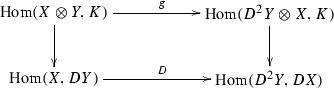  (9.4)

  whose vertical arrows come from (9.1).

• (iii) In any Grothendieck–Verdier category, there exist right and left internal $\mathrm{Hom }$’s. More precisely, if one sets

  $$\begin{aligned} \underline{\mathrm{Hom }}(X,Z)&= D^{-1}(DZ\otimes X),\end{aligned}$$

  (9.5)
  $$\begin{aligned} \underline{\mathrm{Hom }}^{\prime }(Y,Z)&= D(Y\otimes D^{-1}Z) \end{aligned}$$

  (9.6)

  then(9.1) and (9.2) yield functorial isomorphisms

  $$\begin{aligned}&\mathrm{Hom }(X\otimes Y,Z)\mathop {\longrightarrow }\limits ^{\simeq }\mathrm{Hom }(Y, \underline{\mathrm{Hom }}(X,Z)),\end{aligned}$$

  (9.7)
  $$\begin{aligned}&\mathrm{Hom }(X\otimes Y,Z)\mathop {\longrightarrow }\limits ^{\simeq }\mathrm{Hom }(X, \underline{\mathrm{Hom }}^{\prime }(Y,Z)). \end{aligned}$$

  (9.8)

• (iv) From (9.1) and (9.2), one gets canonical isomorphisms

  $$\begin{aligned} D{1\!\!1}\mathop {\longrightarrow }\limits ^{\simeq } K, \quad \quad D^{-1}{1\!\!1}\mathop {\longrightarrow }\limits ^{\simeq } K. \end{aligned}$$

  (9.9)

  and therefore canonical isomorphisms

  $$\begin{aligned}&{1\!\!1}\mathop {\longrightarrow }\limits ^{\simeq } D^2{1\!\!1},\end{aligned}$$

  (9.10)
  $$\begin{aligned}&K\mathop {\longrightarrow }\limits ^{\simeq } D^2K \end{aligned}$$

  (9.11)

  (the latter is the composition $K\mathop {\longrightarrow }\limits ^{\simeq } D{1\!\!1}\mathop {\longrightarrow }\limits ^{\simeq } D^2D^{-1}{1\!\!1}\mathop {\longrightarrow }\limits ^{\simeq } D^2K$).

1.1.3 $D^2$ as a monoidal equivalence

By (9.3), for each $X,Y_1,Y_2\in \mathcal{M }$, one has a canonical isomorphism

$$\begin{aligned} \mathrm{Hom }(X\otimes Y_1\otimes Y_2, K )\mathop {\longrightarrow }\limits ^{\simeq }\mathrm{Hom }(D^2(Y_1\otimes Y_2)\otimes X, K ). \end{aligned}$$

(9.12)

On the other hand, writing $X\otimes Y_1\otimes Y_2$ as $(X\otimes Y_1)\otimes Y_2$ and applying (9.3) twice, one gets an isomorphism

$$\begin{aligned} \mathrm{Hom }(X\otimes Y_1\otimes Y_2, K )\mathop {\longrightarrow }\limits ^{\simeq }\mathrm{Hom }(D^2Y_1\otimes D^2Y_2\otimes X, K ). \end{aligned}$$

(9.13)

Combining (9.12) and (9.13), one gets a functorial isomorphism

$$\begin{aligned} \mathrm{Hom }(D^2(Y_1\otimes Y_2)\otimes X, K )\mathop {\longrightarrow }\limits ^{\simeq }\mathrm{Hom }(D^2Y_1\otimes D^2Y_2\otimes X, K ), \quad X,Y_1,Y_2\in \mathcal{M }.\nonumber \\ \end{aligned}$$

(9.14)

Using Yoneda’s lemma and the isomorphism

$$\begin{aligned} \mathrm{Hom }(Z\otimes X,K)\mathop {\longrightarrow }\limits ^{\simeq }\mathrm{Hom }(Z,DX) \end{aligned}$$

we see that the isomorphism (9.14) comes from a unique functorial isomorphism

$$\begin{aligned} D^2(Y_1\otimes Y_2)\mathop {\longrightarrow }\limits ^{\simeq } D^2Y_1\otimes D^2Y_2 , \quad Y_1,Y_2\in \mathcal{M }. \end{aligned}$$

(9.15)

Proposition 9.13

The isomorphism (9.15) defines a monoidal structure on the functor $D^2:\mathcal{M }\mathop {\longrightarrow }\limits ^{\simeq }\mathcal{M }$.

A proof is given in [16, §11.1]. We do not use Proposition 9.13 in the main body of this article.

1.2 Pivotal structures on Grothendieck–Verdier categories

1.2.1 The notion of a pivotal structure

Definition 9.14

A pivotal structure  on a Grothendieck–Verdier category $\mathcal{M }$ is a functorial isomorphism

$$\begin{aligned} \psi _{X,Y}:\mathrm{Hom }(X\otimes Y,K )\mathop {\longrightarrow }\limits ^{\simeq }\mathrm{Hom }(Y\otimes X,K ), \quad X,Y\in \mathcal{M }\end{aligned}$$

(9.16)

such that

$$\begin{aligned}&\displaystyle \psi _{X\otimes Y,Z}\circ \psi _{Y\otimes Z,X}\circ \psi _{Z\otimes X,Y}=\mathrm{id }, \quad X,Y\in \mathcal{M };\end{aligned}$$

(9.17)

$$\begin{aligned}&\displaystyle \psi _{X,Y}\circ \psi _{Y,X}=\mathrm{id }, \quad X,Y\in \mathcal{M }. \end{aligned}$$

(9.18)

In particular, one has the notion of a pivotal structure on an r-category (which can be considered as a Grothendieck–Verdier category with $K={1\!\!1}$).

Definition 9.15

A pivotal Grothendieck–Verdier category is a Grothendieck–Verdier category with a pivotal structure. A pivotal r-category  is an r-category with a pivotal structure.

The name “pivotal category” goes back to [29, Definition 1.3].

Example 9.16

A symmetric Grothendieck–Verdier category has a canonical pivotal structure: The isomorphisms $\mathrm{Hom }(M\otimes N,K)\mathop {\longrightarrow }\limits ^{\simeq }\mathrm{Hom }(N\otimes M,K)$ are induced by the symmetry isomorphisms $M\otimes N\mathop {\longrightarrow }\limits ^{\simeq }N\otimes M$. In particular, one thus gets a canonical pivotal structure on the Grothendieck–Verdier category $({\fancyscript{D}}(X),K_X)$ from Example 9.5.

Lemma 9.17

Let $\mathcal{M }$ be a Grothendieck–Verdier category and $\psi$ an isomorphism (9.16) satisfying (9.17). Then $\psi$ satisfies (9.18) if and only if $\psi _{K,{1\!\!1}}=\mathrm{id }$.

Proof

Setting $Z={1\!\!1}$ in (9.17), we see that (9.18) holds if and only if the isomorphism $\psi _{X,{1\!\!1}}:\mathrm{Hom }(X,K )\rightarrow \mathrm{Hom }(X,K )$ equals the identity for all $X$. By Yoneda’s lemma, this happens if and only if $\psi _{K,{1\!\!1}}=\mathrm{id }$. $\square$

Corollary 9.18

If $\mathcal{M }$ is an r-category, then (9.17) implies (9.18).

Remark 9.19

By (9.17) and (9.18), a pivotal structure on a Grothendieck–Verdier category defines for any integers $n\ge m\ge 1$ a canonical isomorphism

$$\begin{aligned} \mathrm{Hom }(X_1\otimes \cdots \otimes X_n,K)\mathop {\longrightarrow }\limits ^{\simeq }\mathrm{Hom }(X_m\otimes \cdots \otimes X_n\otimes X_1\otimes \cdots \otimes X_{m-1},K) \end{aligned}$$

for all $X_1,X_2,\ldots ,X_n\in \mathcal{M }$.

1.2.2 Pivotal structures and isomorphisms $\mathrm{id }\mathop {\longrightarrow }\limits ^{\simeq } D^2$

Remark 9.20

By (9.1)–(9.2) and Yoneda’s lemma, a functorial isomorphism (9.16) is the same as an isomorphism $D^{-1}\mathop {\longrightarrow }\limits ^{\simeq } D$ or equivalently an isomorphism $\mathrm{id }\mathop {\longrightarrow }\limits ^{\simeq } D^2$.

Remark 9.20 yields an injective map from the set of pivotal structures on a Grothendieck–Verdier category $\mathcal{M }$ to the set of isomorphisms $f:\mathrm{id }\mathop {\longrightarrow }\limits ^{\simeq } D^2$.

Proposition 9.21

An isomorphism $f:\mathrm{id }\mathop {\longrightarrow }\limits ^{\simeq } D^2$ belongs to the image of this map if and only if it satisfies the following conditions:

• (i) $f$ is monoidal;

• (ii) $f_K:K\mathop {\longrightarrow }\limits ^{\simeq } D^2K$ equals the isomorphism (9.11).

A proof is given in [16, §13]. We do not use Proposition 9.21 in the main body of this article.

Remarks 9.22

• (i) If $\mathcal{M }$ is an r-category, then condition (ii) from Proposition 9.21 clearly follows from condition (i). For arbitrary Grothendieck–Verdier categories, this is false, see [16, Remark 5.8(i)].

• (ii) By the previous remark, in the case of r-categories a pivotal structure can equivalently be defined to be a monoidal isomorphism $f:\mathrm{id }\mathop {\longrightarrow }\limits ^{\simeq } D^2$. It is this definition that was used in works on rigid monoidal categories (e.g., see [28, Definition 2.7]).

• (iii) Here is a way to combine the two conditions on $f$ from Proposition 9.21 into one. Let $\mathfrak{A }$ be the 2-groupoid of pairs consisting of a monoidal category and an object in it. A Grothendieck–Verdier category $(\mathcal{M },K)$ is an object in $\mathfrak{A }$. The monoidal structure on $D^2$ and the isomorphism $K\mathop {\longrightarrow }\limits ^{\simeq } D^2(K)$ defined in Remark 9.12(iv) allow us to consider $D^2$ as a 1-automorphism of $(\mathcal{M },K)\in \mathfrak{A }$. The two conditions on $f$ from Proposition 9.21 mean that $f:\mathrm{id }\mathop {\longrightarrow }\limits ^{\simeq } D^2$ is a 2-isomorphism in $\mathfrak{A }$.

1.2.3 The canonical pivotal structure on ${\fancyscript{D}}(G)$ and ${\fancyscript{D}}_G(G)$

Example 9.23

We will write $\mathcal{M }$ for one of the r-categories ${\fancyscript{D}}(G)$ and ${\fancyscript{D}}_G(G)$ (cf. Example 9.9). Let us give a description of $\mathrm{Hom }(M_1*\cdots *M_n,{1\!\!1})$, $M_i\in \mathcal{M }$, which makes the pivotal structure on $\mathcal{M }$ obvious. First,

$$\begin{aligned} \mathrm{Hom }(M_1*\cdots *M_n,{1\!\!1})=\mathrm{Hom }(1^* (M_1*\cdots *M_n), {\overline{\mathbb{Q }}_\ell }), \end{aligned}$$

(9.19)

where $1:\mathrm{Spec }\,k\mathop {\longrightarrow }\limits ^{}G$ is the unit of $G$ (of course, in the case $\mathcal{M }={\fancyscript{D}}_G(G)$ the right-hand side of (9.19) should be understood as $\mathrm{Hom }$ in the category ${\fancyscript{D}}_G (\mathrm{Spec }\,k)$). Now, define $Z_n\subset G^n$ by the equation $g_1\ldots g_n=1$, and let $\pi _1,\ldots ,\pi _n:Z_n\mathop {\longrightarrow }\limits ^{}G$ be the projections. Then by proper base change,

$$\begin{aligned} 1^* (M_1*\cdots *M_n)=p_! (\pi _1^*M_1\otimes \cdots \otimes \pi _n^*M_n), \quad \quad p:Z_n\mathop {\longrightarrow }\limits ^{}\mathrm{Spec }\,k .\qquad \end{aligned}$$

(9.20)

Combining (9.19) with (9.20) and using the invariance of $Z_n\subset G^n$ with respect to cyclic permutations of the $n$ coordinates, we get a canonical isomorphism

$$\begin{aligned} \mathrm{Hom }(M_1*\cdots *M_n,{1\!\!1}) \mathop {\longrightarrow }\limits ^{\simeq } \mathrm{Hom }(M_2*\cdots *M_n*M_1,{1\!\!1}) \end{aligned}$$

whose $n$-th power (in the obvious sense) equals the identity .

It is easy to see that the isomorphisms $\mathrm{Hom }(M_1*M_2,{1\!\!1})\mathop {\longrightarrow }\limits ^{\simeq }\mathrm{Hom }(M_2*M_1,{1\!\!1})$ that we obtain in the case $n=2$ of this construction define a pivotal structure on the r-category $\mathcal{M }$ (which is either ${\fancyscript{D}}(G)$ or ${\fancyscript{D}}_G(G)$).

Remarks 9.24

• (i) The Grothendieck–Verdier category from Example 9.11 has a canonical pivotal structure (in the spirit of Example 9.23).

• (ii) By Remark 9.20, the pivotal structure on ${\fancyscript{D}}(G)$ (respectively, ${\fancyscript{D}}_G(G)$) from Example 9.23 yields an isomorphism $f:\mathrm{Id }\mathop {\longrightarrow }\limits ^{\simeq } (\mathbb{D }_G^-)^2$. Let us compute it.

Lemma 9.25

The isomorphism $f:\mathrm{Id }\mathop {\longrightarrow }\limits ^{\simeq }(\mathbb{D }_G^-)^2$ coming from the pivotal structure of Example 9.23 is equal to the composition

$$\begin{aligned} \mathrm{Id }\mathop {\longrightarrow }\limits ^{\simeq } \mathbb{D }_G^2 \mathop {\longrightarrow }\limits ^{\simeq } (\iota ^*)^2\circ \mathbb{D }_G^2 \mathop {\longrightarrow }\limits ^{\simeq } \iota ^*\circ \mathbb{D }_G\circ \iota ^*\circ \mathbb{D }_G=(\mathbb{D }_G^-)^2, \end{aligned}$$

where the first isomorphism is the standard one and the other two come from the natural identifications $(\iota ^*)^2\cong \mathrm{Id }$ and $\mathbb{D }_G\circ \iota ^*\cong \iota ^*\circ \mathbb{D }_G$.

This lemma will be deduced in Sect. 9.2.5 from a more general Lemma 9.29.

1.2.4 Quasi-pivotal structures

Let ${\fancyscript{C}}$ be a category and $\Phi :{\fancyscript{C}}\times {\fancyscript{C}}\mathop {\longrightarrow }\limits ^{}\mathcal{S }{}ets$ a dualizing functor (see Definition 9.1). Let $D$ be the duality functor with respect to $\Phi$, i.e., $\mathrm{Hom }(X,DY)=\Phi (X,Y)$ for $X,Y\in {\fancyscript{C}}$.

Definition 9.26

A quasi-pivotal structure on $\Phi$ is a functorial family of isomorphisms

$$\begin{aligned} \psi _{X,Y}:\Phi (X,Y)\mathop {\longrightarrow }\limits ^{\simeq }\Phi (Y,X), \qquad X,Y\in {\fancyscript{C}}. \end{aligned}$$

Remark 9.27

If $\psi$ is a quasi-pivotal structure on $\Phi$, then for $X,Y\in {\fancyscript{C}}$ we obtain a functorial isomorphism

$$\begin{aligned} \begin{aligned} \mathrm{Hom }(X,Y)&\mathop {\longrightarrow }\limits ^{D}\mathrm{Hom }(DY,DX)= \Phi (DY,X) \\&\xrightarrow {\psi _{DY,X}\ }\Phi (X,DY)= \mathrm{Hom }(X,D^2 Y) \end{aligned} \end{aligned}$$

and hence a functorial isomorphism $Y\mathop {\longrightarrow }\limits ^{\simeq }D^2 Y$. This defines a bijection between quasi-pivotal structures on $\Phi$ and isomorphisms of functors $\mathrm{Id }_{{\fancyscript{C}}}\mathop {\longrightarrow }\limits ^{\simeq }D^2$.

From now on, we assume that we are given a triple $({\fancyscript{C}},\Phi ,\psi )$, where ${\fancyscript{C}}$ is a category, $\Phi :{\fancyscript{C}}\times {\fancyscript{C}}\mathop {\longrightarrow }\limits ^{}\mathcal{S }{}ets$ is a dualizing functor, and $\psi$ is a quasi-pivotal structure on $\Phi$. Suppose moreover that we are given an action of $\mathbb{Z }/2\mathbb{Z }$ on $({\fancyscript{C}},\Phi ,\psi )$. We write $\tau :{\fancyscript{C}}\mathop {\longrightarrow }\limits ^{\sim }{\fancyscript{C}}$ for the autoequivalence defined by $1\in \mathbb{Z }/2\mathbb{Z }$.

Remarks 9.28

• (1) The functor $\Phi ^\tau :(X,Y)\longmapsto \Phi (\tau X,Y)$ is also dualizing, and the corresponding duality functor is $\tau ^{-1}\circ D\cong \tau \circ D$, where $D$ is the duality functor with respect to $\Phi$.

• (2) The functor $D$ is $(\mathbb{Z }/2\mathbb{Z })$-equivariant, so there is a natural isomorphism

  $$\begin{aligned} \tau \circ D\mathop {\longrightarrow }\limits ^{\simeq }D\circ \tau . \end{aligned}$$

• (3) The composition

  $$\begin{aligned} \psi ^\tau _{X,Y} : \Phi (\tau X,Y) \mathop {\longrightarrow }\limits ^{\simeq } \Phi (X,\tau Y) \mathop {\longrightarrow }\limits ^{\simeq } \Phi (\tau Y,X), \qquad X,Y\in {\fancyscript{C}}, \end{aligned}$$

  defines a quasi-pivotal structure on $\Phi ^\tau$, where the first isomorphism comes from the $\mathbb{Z }/2\mathbb{Z }$-equivariant structure on $\Phi$ and the second one is $\psi _{X,\tau Y}\,$.

Lemma 9.29

The isomorphism $\mathrm{Id }_{{\fancyscript{C}}}\mathop {\longrightarrow }\limits ^{\simeq }(\tau \circ D)^2$ coming from the quasi-pivotal structure described in Remark 9.28(3) via the construction of Remark 9.27 is equal to the composition

$$\begin{aligned} \mathrm{Id }_{{\fancyscript{C}}}\mathop {\longrightarrow }\limits ^{\simeq } D^2 \mathop {\longrightarrow }\limits ^{\simeq } \tau ^2\circ D^2 \mathop {\longrightarrow }\limits ^{\simeq } (\tau \circ D)^2, \end{aligned}$$

where the first isomorphism corresponds to $\psi$ as in Remark 9.27, the second one comes from the natural identification $\mathrm{Id }_{{\fancyscript{C}}}\cong \tau ^2$, and the third one is induced by the isomorphism $\tau \circ D\mathop {\longrightarrow }\limits ^{\simeq }D\circ \tau$ of Remark 9.28(2).

The proof is completely straightforward, so we omit it.

1.2.5 Proof of Lemma 9.25

Let us specialize Sect. 9.2.4 to the following setting. Take ${\fancyscript{C}}$ to be either ${\fancyscript{D}}(G)$ or ${\fancyscript{D}}_G(G)$, define $\Phi (M_1,M_2)=\mathrm{Hom }(M_1\otimes M_2,K_G)$, where $K_G\in {\fancyscript{C}}$ is the dualizing complex, and let $\psi$ be induced by the standard symmetry isomorphism $M_1\otimes M_2\mathop {\longrightarrow }\limits ^{\simeq }M_2\otimes M_1$. The action of $\mathbb{Z }/2\mathbb{Z }$ on the triple $({\fancyscript{C}},\Phi ,\psi )$ comes from $\tau :=\iota ^*$, where $\iota :G\mathop {\longrightarrow }\limits ^{}G$ is the inversion map.

We claim that the new duality functor $\Phi ^\tau$ can be naturally identified with the functor $(M_1,M_2)\longmapsto \mathrm{Hom }(M_1*M_2,{1\!\!1})$, so that $\psi ^\tau$ becomes identified with the pivotal structure defined in Example 9.23. Indeed, with the notation of Example 9.23, we can identify $G$ with $Z_2\subset G\times G$ via the map $g\mapsto (g^{-1},g)$. Under this identification, $\pi _1$ becomes $\iota$ and $\pi _2$ becomes the identity map on $G$. Hence,

$$\begin{aligned} \mathrm{Hom }(M_1*M_2,{1\!\!1})\mathop {\longrightarrow }\limits ^{\simeq }\mathrm{Hom }(p_!(\iota ^*M_1\otimes M_2),{\overline{\mathbb{Q }}_\ell })\mathop {\longrightarrow }\limits ^{\simeq }\mathrm{Hom }(\iota ^*M_1\otimes M_2,K_G). \end{aligned}$$

This implies that $\Phi ^\tau (M_1,M_2)=\mathrm{Hom }(M_1*M_2,{1\!\!1})$, and the fact that $\psi ^\tau$ coincides with the pivotal structure described in Example 9.23 follows from the construction. Applying Lemma 9.29 completes the proof.

1.3 Braided Grothendieck–Verdier categories

1.3.1 The functors $D^2$ and $D^4$

The next result is proved in [16, Lemma 6.8].

Lemma 9.30

Let $(\mathcal{M },K,\beta )$ be a braided Grothendieck–Verdier category, and let $\varphi ^\pm :D^{-1}\mathop {\longrightarrow }\limits ^{\simeq }D$ be the isomorphisms induced by the compositions

$$\begin{aligned} \begin{aligned} \mathrm{Hom }(Y,D^{-1}X)&\mathop {\longrightarrow }\limits ^{\simeq } \mathrm{Hom }(X\otimes Y,K) \xrightarrow {\ \ (\beta ^\pm _{Y,X})^*\ \ } \mathrm{Hom }(Y\otimes X,K) \\&\mathop {\longrightarrow }\limits ^{\simeq } \mathrm{Hom }(Y,DX) \end{aligned} \end{aligned}$$

for all $X,Y\in \mathcal{M }$, where $\beta _{X,Y}^+:=\beta _{X,Y}$ and $\beta _{X,Y}^-:=\beta _{Y,X}^{-1}$. Then

$$\begin{aligned} D(\varphi ^\pm _X) = (\varphi ^\mp _{DX})^{-1} \quad \text{ for } \text{ all } X\in \mathcal{M }. \end{aligned}$$

Definition 9.31

If $(\mathcal{M },K,\beta )$ is a braided Grothendieck–Verdier category, we define isomorphisms of functors $\vartheta ^\pm :\mathrm{Id }_{\mathcal{M }}\mathop {\longrightarrow }\limits ^{\simeq }D^2$ as follows:

$$\begin{aligned} \vartheta ^\pm _X = \varphi ^\pm _{DX} = D(\varphi ^\mp _X)^{-1} : X\mathop {\longrightarrow }\limits ^{\simeq }D^2 X \qquad \forall \,X\in \mathcal{M }, \end{aligned}$$

where the second equality holds by the lemma above.

Remark 9.32

In general, the isomorphisms $\vartheta ^\pm$ are not monoidal.

Lemma 9.33

Let $(\mathcal{M },K,\beta )$ be a braided Grothendieck–Verdier category.

Then the monoidal functor $D^2:\mathcal{M }\mathop {\longrightarrow }\limits ^{\sim }\mathcal{M }$ is braided.

This result is [16, Proposition 6.1(i)]. The lemma implies that the functor $D^4:\mathcal{M }\mathop {\longrightarrow }\limits ^{\sim }\mathcal{M }$ is also braided. Note that we can consider $\vartheta ^+\vartheta ^-$ as an isomorphism of functors between $\mathrm{Id }_{\mathcal{M }}$ and $D^4$.

Lemma 9.34

In any braided Grothendieck–Verdier category $(\mathcal{M },K,\beta )$, the isomorphism $\vartheta ^+\vartheta ^- : \mathrm{Id }_{\mathcal{M }}\mathop {\longrightarrow }\limits ^{\simeq }D^4$ is monoidal. One has $\vartheta ^-\vartheta ^+=\vartheta ^+\vartheta ^-$.

For the proof, see Definition 6.11 and Remark 6.12 in [16].

1.3.2 Pivotal structures and twists

Let us recall the following.

Definition 9.35

If $(\mathcal{M },\beta )$ is a braided monoidal category, a twist on $(\mathcal{M },\beta )$ is an automorphism $\theta :\mathrm{Id }_{\mathcal{M }}\mathop {\longrightarrow }\limits ^{\simeq }\mathrm{Id }_{\mathcal{M }}$ of the identity functor satisfying

$$\begin{aligned} \theta _{X\otimes Y} = \beta _{Y,X}\circ \beta _{X,Y}\circ (\theta _X\otimes \theta _Y) \qquad \forall \,X,Y\in \mathcal{M }. \end{aligned}$$

Now suppose $(\mathcal{M },K,\beta )$ is a braided Grothendieck–Verdier category equipped with a pivotal structure $\psi$. There exists a unique automorphism $\theta$ of $\mathrm{Id }_{\mathcal{M }}$ such that for all $X,Y\in \mathcal{M }$ the isomorphism

$$\begin{aligned} \mathrm{Hom }(Y,D^{-1}X)\mathop {\longrightarrow }\limits ^{\simeq }\mathrm{Hom }(Y,D^{-1}X), \qquad g\longmapsto g \circ \theta _Y, \end{aligned}$$

is equal to the composition

$$\begin{aligned}&\mathrm{Hom }(Y,D^{-1}X) \mathop {\longrightarrow }\limits ^{\simeq } \mathrm{Hom }(X\otimes Y,K) \xrightarrow {\ \ \psi _{X,Y}\ \ } \mathrm{Hom }(Y\otimes X,K)\\&\quad \xrightarrow {(\beta _{Y,X}^{-1})^*\ \ } \mathrm{Hom }(X\otimes Y, K) \mathop {\longrightarrow }\limits ^{\simeq } \mathrm{Hom }(Y,D^{-1}X). \end{aligned}$$

Remark 9.36

It is clear that $\psi$ can be expressed in terms of $\theta$ as follows:

$$\begin{aligned} \psi _{X,Y} = \beta _{Y,X}^*\circ (\mathrm{id }_X\otimes \theta _Y)^* \end{aligned}$$

as isomorphisms

$$\begin{aligned} \mathrm{Hom }(X\otimes Y,K) \mathop {\longrightarrow }\limits ^{\simeq } \mathrm{Hom }(X\otimes Y,K) \mathop {\longrightarrow }\limits ^{\simeq } \mathrm{Hom }(Y\otimes X,K) \end{aligned}$$

for all $X,Y\in \mathcal{M }$.

Lemma 9.37

The map $\psi \mapsto \theta$ constructed above is a bijection between the set of pivotal structures on $(\mathcal{M },K)$ and the set of twists $\theta$ on $(\mathcal{M },\beta )$ satisfying $\theta _K=\mathrm{id }_K$.

For the proof, see Proposition 7.1 and Remark 7.2 in [16].

Remarks 9.38

• (1) In the situation of Lemma 9.37, let $f:\mathrm{Id }_{\mathcal{M }}\mathop {\longrightarrow }\limits ^{\simeq }D^2$ be the monoidal isomorphism corresponding to $\psi$ as in Remark 9.20 (see also Proposition 9.21). Unwinding the definitions, one sees that in terms of $f$, the twist corresponding to $\psi$ is given by $\theta =(\vartheta ^+)^{-1}\circ f$, where $\vartheta ^+:\mathrm{Id }_{\mathcal{M }}\mathop {\longrightarrow }\limits ^{\simeq }D^2$ is the isomorphism constructed in Definition 9.31.

• (2) Let $(\mathcal{M },K,\beta )$ be a braided Grothendieck–Verdier category, and let $\theta$ be a twist on $(\mathcal{M },\beta )$ such that $\theta _K=\mathrm{id }_K$. If one defines $\theta ^{\prime }_X=D^{-1}(\theta _{DX})$ for all $X\in \mathcal{M }$, then $\theta ^{\prime }$ is also a twist on $(\mathcal{M },\beta )$ satisfying $\theta ^{\prime }_K=\mathrm{id }_K$ [16, Prop. 7.3(iii)–(iv)].

• (3) The map $\theta \mapsto \theta ^{\prime }$ is an involution of the set of twists of $(\mathcal{M },\beta )$ that act as the identity on $K$ [16, Prop. 7.3(i)–(ii)].

• (4) The involution $\theta \mapsto \theta ^{\prime }$ can be described in different terms [16, Prop. 7.3(v)]. Let $\psi ,\psi ^{\prime }$ be the pivotal structures corresponding to $\theta$ and $\theta ^{\prime }$, and let $f,f^{\prime }:\mathrm{Id }_{\mathcal{M }}\mathop {\longrightarrow }\limits ^{\simeq }D^2$ be the monoidal isomorphisms corresponding to $\psi ,\psi ^{\prime }$. Then $ff^{\prime }:\mathrm{Id }_{\mathcal{M }}\mathop {\longrightarrow }\limits ^{\simeq }D^4$ is equal to the monoidal isomorphism $\vartheta ^+\vartheta ^-:\mathrm{Id }_{\mathcal{M }}\mathop {\longrightarrow }\limits ^{\simeq }D^4$ of Lemma 9.34.

1.4 Ribbon Grothendieck–Verdier categories

Definition 9.39

A ribbon structure on a braided Grothendieck–Verdier category $(\mathcal{M },K,\beta )$ is a twist $\theta$ on $(\mathcal{M },\beta )$ such that

$$\begin{aligned} \theta _X=D^{-1}(\theta _{DX})\quad \text{ for } \text{ all } X\in \mathcal{M }. \end{aligned}$$

(9.21)

A ribbon Grothendieck–Verdier category is a braided Grothendieck–Verdier category with a ribbon structure. A ribbon r-category is an r-category with a ribbon structure.

Remark 9.40

The identity (9.21) holds if and only if for any $X,Y\in \mathcal{M }$ and $B:X\otimes Y\mathop {\longrightarrow }\limits ^{} K$ one has

$$\begin{aligned} B\circ (\mathrm{id }_X\otimes \theta _Y)=B\circ (\theta _X\otimes \mathrm{id }_Y). \end{aligned}$$

(9.22)

Note that unlike (9.21), formula (9.22) makes sense in any braided category with a fixed object $K$ ($K$ does not have to be dualizing and $\mathcal{M }$ does not have to be Grothendieck–Verdier). We do not know whether condition (9.22) is really interesting in this generality.

Lemma 9.41

A twist $\theta$ satisfies (9.21) if and only if $\theta _K=\mathrm{id }_K$ and $\theta ^{\prime }=\theta$, where $\theta ^{\prime }$ is defined in Remark 9.38(2).

Proof

We only have to show that the equality $\theta _K=\mathrm{id }_K$ follows from (9.21). This is clear because $K=D{1\!\!1}$ and $\theta _{{1\!\!1}}=\mathrm{id }_{{1\!\!1}}$. $\square$

Corollary 9.42

The correspondence between twists and pivotal structures $($see Lemma 9.37$)$ induces a bijection between ribbon structures on $(\mathcal{M },K,\beta )$ and those pivotal structures on $(\mathcal{M },K)$ for which the corresponding monoidal isomorphism $f:\mathrm{Id }_{\mathcal{M }}\mathop {\longrightarrow }\limits ^{\simeq }D^2$ is invariant under the involution $f\mapsto f^{\prime }$ from Remark 9.38(4).

Proof

This follows from Lemma 9.41 and Remark 9.38(4). $\square$

1.5 The canonical ribbon structure on ${\fancyscript{D}}_G(G)$

The r-category $({\fancyscript{D}}_G(G),*)$ has a natural ribbon structure. For an arbitrary algebraic group $G$, it is described in Appendix 10 below. In this subsection we define it for algebraic groups $G$ such that $G^\circ$ is unipotent. This assumption allows us to use the ad hoc construction of ${\fancyscript{D}}_G(G)$ given in Definition 2.3.

Definition 9.43

(Braiding on ${\fancyscript{D}}_G(G)$) Let $M,N\in {\fancyscript{D}}_G(G)$, then the braiding $\beta _{M,N}:M*N\mathop {\longrightarrow }\limits ^{\simeq } N*M$ is defined as follows. Consider the commutative diagram

where $\tau (g,h):=(h,g)$ and $\xi (g,h):=(g,g^{-1}hg)$. We have $M*N=\mu _!(M\boxtimes N)$, and the above diagram shows that $N*M=(\mu \tau )_!(M\boxtimes N)=\mu _!\xi _!(M\boxtimes N)$. We define $\beta _{M,N}:\mu _!(M\boxtimes N)\mathop {\longrightarrow }\limits ^{\simeq }\mu _!\xi _!(M\boxtimes N)$ by $\beta _{M,N}:=\mu _!(f)$, where $f:M\boxtimes N\mathop {\longrightarrow }\limits ^{\simeq }\xi _!(M\boxtimes N)$ comes from the $G$-equivariant structure on $N$.

Remark 9.44

Checking the axioms of a braiding for $\beta$ is straightforward and is similar to the well-known case where $G$ is finite. In this case ${\fancyscript{D}}_G(G)$ is the derived category of modules over the so-called quantum double of the group algebra of $G$ (see, e.g., §3.2 of [9]). These modules form a braided category which is not symmetric unless $|G|=1$.

Definition 9.45

(Twist on ${\fancyscript{D}}_G(G)$) Let $c:G\times G\rightarrow G$ be the conjugation action morphism $c(g,h)=ghg^{-1}$, let $p_2:G\times G\rightarrow G$ denote the second projection, and let $\Delta :G\rightarrow G\times G$ denote the diagonal. Then $c\circ \Delta =\mathrm{id }_G=p_2\circ \Delta$. For each $M\in {\fancyscript{D}}_G(G)$, the $G$-equivariant structure on $M$ yields an isomorphism $p_2^*M\mathop {\longrightarrow }\limits ^{\simeq } c^*M$. Pulling it back by $\Delta$, we get an isomorphism $\theta _M:M= \Delta ^*p_2^*M\mathop {\longrightarrow }\limits ^{\simeq }\Delta ^*c^*M=M$.

By construction, $\theta$ is an automorphism of the identity functor on ${\fancyscript{D}}_G(G)$, and one can check that it is related to the braiding $\beta$ of Definition 9.43 as follows:

$$\begin{aligned} \theta _{M*N} = \beta _{N,M}\circ \beta _{M,N}\circ (\theta _M*\theta _N) \qquad \forall \, M,N\in {\fancyscript{D}}_G(G). \end{aligned}$$

In fact, this follows from part (a) of

Proposition 9.46

• (a) If the r-category ${\fancyscript{D}}_G(G)$ is equipped with the pivotal structure of Example 9.23 and the braiding of Definition 9.43, the corresponding twist $($cf. Lemma 9.37$)$ is the automorphism $\theta$ constructed in Definition 9.45.

• (b) The twist $\theta$ is a ribbon structure on the braided r-category $({\fancyscript{D}}_G(G),\beta )$.

By Remark 9.36, the proposition follows at once from the next two lemmas.

Lemma 9.47

If $M,N\in {\fancyscript{D}}_G(G)$, then the isomorphism

$$\begin{aligned} \psi _{M,N} : \mathrm{Hom }(M*N,{1\!\!1}) \mathop {\longrightarrow }\limits ^{\simeq } \mathrm{Hom }(N*M,{1\!\!1}) \end{aligned}$$

from Example 9.23 is equal to the pullback map via the composition

$$\begin{aligned} (\mathrm{id }_M*\theta _N)\circ \beta _{N,M} : N*M \mathop {\longrightarrow }\limits ^{\simeq } M*N. \end{aligned}$$

Lemma 9.48

For all $M\in {\fancyscript{D}}_G(G)$, we have $\theta _{\mathbb{D }_G^-M}=\mathbb{D }_G^-(\theta _M)$.

For Lemma 9.48 we refer to [25, Proposition 7.2].

Proof of Lemma 9.47

We use the notation of Example 9.23. In particular,

$$\begin{aligned} Z_2 = \bigl \{ (g,h)\in G\times G \,\big \vert \,gh=1 \bigr \}, \end{aligned}$$

$\pi _1,\pi _2:Z_2\mathop {\longrightarrow }\limits ^{}G$ are the two projections, and $p:Z_2\mathop {\longrightarrow }\limits ^{}\mathrm{Spec }\,k$ is the structure morphism. The composition

$$\begin{aligned} \begin{aligned} \mathrm{Hom }(M*N,1_*{\overline{\mathbb{Q }}_\ell })&\mathop {\longrightarrow }\limits ^{\simeq } \mathrm{Hom }(1^*(M*N),{\overline{\mathbb{Q }}_\ell }) \\&\mathop {\longrightarrow }\limits ^{\simeq } \mathrm{Hom }\bigl ( p_!(\pi _1^*(M)\otimes \pi _2^*(N)),{\overline{\mathbb{Q }}_\ell }\bigr ) \end{aligned} \end{aligned}$$

yields an identification³³

$$\begin{aligned} \mathrm{Hom }(M*N,{1\!\!1}) \mathop {\longrightarrow }\limits ^{\simeq } \mathrm{Hom }\bigl ( p_!(\pi _1^*(M)\otimes \pi _2^*(N)),{\overline{\mathbb{Q }}_\ell }\bigr ). \end{aligned}$$

(9.23)

Similarly, we have an identification

$$\begin{aligned} \mathrm{Hom }(N*M,{1\!\!1}) \mathop {\longrightarrow }\limits ^{\simeq } \mathrm{Hom }\bigl ( p_!(\pi _1^*(N)\otimes \pi _2^*(M)),{\overline{\mathbb{Q }}_\ell }\bigr ). \end{aligned}$$

(9.24)

Let $\tau :G\times G\mathop {\longrightarrow }\limits ^{\simeq }G\times G$ and $\xi :G\times G\mathop {\longrightarrow }\limits ^{\simeq }G\times G$ be as in Definition 9.43, that is, $\tau (g,h)=(h,g)$ and $\xi (g,h)=(g,g^{-1}hg)$. Note that both $\tau$ and $\xi$ preserve $Z_2\subset G\times G$; moreover, $\xi \bigl |_{Z_2}=\mathrm{id }_{Z_2}$. We also have $p\circ \tau =p$ and $\pi _1\circ \tau =\pi _2$.

The natural isomorphism $p_!\mathop {\longrightarrow }\limits ^{\simeq }p_!\tau _!$ yields an isomorphism

$$\begin{aligned} p_! ( \pi _1^*(N) \otimes \pi _2^*(M) ) \mathop {\longrightarrow }\limits ^{\simeq } p_! \tau _! ( \pi _1^*(N) \otimes \pi _2^*(M) ) \cong p_!(\pi _1^*(M)\otimes \pi _2^*(N)).\nonumber \\ \end{aligned}$$

(9.25)

The induced isomorphism

$$\begin{aligned} \mathrm{Hom }\bigl ( p_!(\pi _1^*(M)\otimes \pi _2^*(N)),{\overline{\mathbb{Q }}_\ell }\bigr ) \mathop {\longrightarrow }\limits ^{\simeq } \mathrm{Hom }\bigl ( p_!(\pi _1^*(N)\otimes \pi _2^*(M)),{\overline{\mathbb{Q }}_\ell }\bigr ) \end{aligned}$$

coincides with $\psi _{M,N}$ modulo the identifications (9.23) and (9.24).

On the other hand, consider the composition

$$\begin{aligned} N\boxtimes M \xrightarrow {\ \ f\ \ } \xi _! (N\boxtimes M) \xrightarrow {\ \ \xi _!(\mathrm{id }_N\boxtimes \theta _M)\ \ } \xi _!(N\boxtimes M), \end{aligned}$$

(9.26)

where $f:N\boxtimes M\mathop {\longrightarrow }\limits ^{\simeq }\xi _!(N\boxtimes M)$ is the isomorphism coming from the $G$-equivariant structure on $M$, used in Definition 9.43. If we restrict (9.26) to $Z_2$, we obtain the identity automorphism of $\pi _1^*(N)\otimes \pi _2^*(M)$ (here we used the definition of $\theta _M$; recall also that $\xi \bigl |_{Z_2}=\mathrm{id }_{Z_2}$). This implies that the isomorphism $1^*(N*M)\mathop {\longrightarrow }\limits ^{\simeq }1^*(M*N)$ induced by $(\theta _M*\mathrm{id }_N)\circ \beta _{N,M}:N*M\mathop {\longrightarrow }\limits ^{\simeq }M*N$ is equal to the composition (9.25). Equivalently, $\psi _{M,N}$ is equal to the pullback map via the composition

$$\begin{aligned} (\theta _M*\mathrm{id }_N)\circ \beta _{N,M} : N*M \mathop {\longrightarrow }\limits ^{\simeq } M*N. \end{aligned}$$

Finally, observe that since $\theta _{{1\!\!1}}=\mathrm{id }_{{1\!\!1}}$, Lemma 9.48 implies that

$$\begin{aligned} (\theta _M*\mathrm{id }_N)^* = (\mathrm{id }_M*\theta _N)^* : \mathrm{Hom }(M*N,{1\!\!1})\mathop {\longrightarrow }\limits ^{}\mathrm{Hom }(M*N,{1\!\!1}), \end{aligned}$$

which completes the proof. $\square$

1.6 Hecke subcategories of Grothendieck–Verdier categories

The notion of a closed idempotent in a monoidal category was introduced in Definition 3.8(d).

Lemma 9.49

Let $(\mathcal{M },K)$ be a Grothendieck–Verdier category. Let $e\in \mathcal{M }$ be a closed idempotent. Then

$$\begin{aligned} D(e\mathcal{M })&= \mathcal{M }e,\end{aligned}$$

(9.27)

$$\begin{aligned} D(\mathcal{M }e)&= D^2 e\cdot \mathcal{M }. \end{aligned}$$

(9.28)

Note that $D^2 e$ is a closed idempotent: This follows from (9.10) and (9.15). The notation $e\mathcal{M }$ and $\mathcal{M }e$ was introduced in Sect. 3.7.

Proof

Let $\pi :{1\!\!1}\mathop {\longrightarrow }\limits ^{}e$ be an idempotent arrow. If $Y\in e\mathcal{M }$, the morphism $\pi \otimes \mathrm{id }_Y:Y\mathop {\longrightarrow }\limits ^{}e\otimes Y$ is an isomorphism. By (9.1), for every $X\in \mathcal{M }$, the morphism $\mathrm{id }_X\otimes \pi :X\mathop {\longrightarrow }\limits ^{}X\otimes e$ induces a bijection $\mathrm{Hom }(X\otimes e,D Y)\mathop {\longrightarrow }\limits ^{\simeq }\mathrm{Hom }(X,DY)$. Now Proposition 3.12(b) implies that $DY\in \mathcal{M }e$. This proves that

$$\begin{aligned} D(e\mathcal{M })\subset \mathcal{M }e. \end{aligned}$$

(9.29)

Now apply (9.29) to $\mathcal{M }$ equipped with the opposite tensor product. Then the dualization functor equals $D^{-1}$, so we get $D^{-1} (\mathcal{M }e)\subset e\mathcal{M }$, i.e., $\mathcal{M }e\subset D(e\mathcal{M })$. Combining this with (9.29), we get (9.27).

To prove (9.28), apply $D$ to (9.27) and note that $D^2(e\mathcal{M })=D^2 e\cdot \mathcal{M }$ by (9.15).

$\square$

Lemma 9.50

Let $(\mathcal{M },K)$ be a Grothendieck–Verdier category, and let $e\in \mathcal{M }$ be a closed idempotent such that $D^2e\simeq e$.

• (a) We have $D(e\mathcal{M })=\mathcal{M }e$ and $D(\mathcal{M }e)= e\mathcal{M }$.

• (b) $De\in e\mathcal{M }e$ is a dualizing object of the monoidal category $e\mathcal{M }e$, so $(e\mathcal{M }e, De)$ is a Grothendieck–Verdier category.

• (c) The corresponding duality functor $e\mathcal{M }e\mathop {\longrightarrow }\limits ^{\sim }e\mathcal{M }e$ can be identified with the restriction of $D$ to $e\mathcal{M }e$. This identification is canonical as soon as one chooses an idempotent arrow $\pi :{1\!\!1}\mathop {\longrightarrow }\limits ^{}e$.

Proof

Statement (a) follows from Lemma 9.49. Let us prove (b) and (c). By Lemma 3.18, $e\mathcal{M }e$ is a monoidal category. By part (a), $D (e\mathcal{M }e)=e\mathcal{M }e$; in particular, $D (e)\in e\mathcal{M }e$. Fix an idempotent arrow $\pi :{1\!\!1}\mathop {\longrightarrow }\limits ^{}e$. Given $X,Y\in e\mathcal{M }e$, we have canonical isomorphisms

$$\begin{aligned} \mathrm{Hom }(X,DY) \cong \mathrm{Hom }(X\otimes Y,K) \cong \mathrm{Hom }(X\otimes Y\otimes e,K) \cong \mathrm{Hom }(X\otimes Y, De), \end{aligned}$$

where the middle one comes from $\pi :{1\!\!1}\mathop {\longrightarrow }\limits ^{}e$ and the other two come from (9.1). This implies both (b) and (c). $\square$

One can ask which Grothendieck–Verdier categories can be realized as $e\mathcal{M }e$, where $\mathcal{M }$ is an r-category and $e\in \mathcal{M }$ is a closed idempotent such that $D^2e\simeq e$. An answer to this question is given in [16, §9].

1.6.1 Hecke subcategories of pivotal Grothendieck–Verdier categories

Lemma 9.51

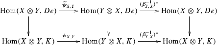
Let $(\mathcal{M },K)$ be a pivotal Grothendieck–Verdier category and $e\in \mathcal{M }$ a closed idempotent. Then $(e\mathcal{M }e, De)$ is a Grothendieck–Verdier category. Moreover, it has a unique pivotal structure $\widetilde{\psi }$ such that for all $X,Y\in e\mathcal{M }e$ and every idempotent arrow $\pi :{1\!\!1}\mathop {\longrightarrow }\limits ^{}e$ the diagram

(9.30)

in which the vertical arrows come from $D\pi :De\mathop {\longrightarrow }\limits ^{}D{1\!\!1}=K$, commutes.

Proof

The first statement follows from Lemma 9.50 because in a pivotal category $D^2\cong \mathrm{Id }$ (see Remark 9.20). Now fix an idempotent arrow $\pi :{1\!\!1}\mathop {\longrightarrow }\limits ^{}e$. Then for every $Z\in \mathcal{M }e$ the map $\mathrm{Hom }(Z,De)\mathop {\longrightarrow }\limits ^{}\mathrm{Hom }(Z,K)$ induced by $D\pi :De\mathop {\longrightarrow }\limits ^{}D{1\!\!1}=K$ is bijective because it equals the composition $\mathrm{Hom }(Z,De)\mathop {\longrightarrow }\limits ^{\simeq } \mathrm{Hom }(Z\otimes e,K)\mathop {\longrightarrow }\limits ^{\simeq }\mathrm{Hom }(Z,K)$, where the first arrow comes from (9.1) and the second one from $\mathrm{id }_Z\otimes \pi :Z\mathop {\longrightarrow }\limits ^{\simeq } Z\otimes e$. Since the vertical arrows in (9.30) are bijections, there is a unique pivotal structure $\widetilde{\psi }$ on $e\mathcal{M }e$ such that the diagram (9.30) corresponding to our fixed idempotent arrow $\pi :{1\!\!1}\mathop {\longrightarrow }\limits ^{}e$ commutes. We have to show that it commutes for any idempotent arrow $\pi ^{\prime } :{1\!\!1}\mathop {\longrightarrow }\limits ^{}e$. By Corollary 3.40, $\pi ^{\prime }=f\circ \pi$ for some $f\in \mathrm{Aut }e$, so it remains to show that the map

$$\begin{aligned} \widetilde{\psi }_{X,Y}:\mathrm{Hom }(X\otimes Y,De)\mathop {\longrightarrow }\limits ^{}\mathrm{Hom }(Y\otimes X,De), \quad X,Y\in e\mathcal{M }e \end{aligned}$$

(9.31)

commutes with $\mathrm{End }e$ acting on both sides of (9.31) via $D:\mathrm{End }e\mathop {\longrightarrow }\limits ^{}\mathrm{End }(De)$. It is easy to check that this action of $\mathrm{End }e$ equals the one that comes from the map $\varphi :\mathrm{End }e\mathop {\longrightarrow }\limits ^{}\mathrm{End }X$ ($\varphi$ is defined because $e$ is a unit object of the monoidal category $e\mathcal{M }e$ and $X\in e\mathcal{M }e$). So the commutation of $\widetilde{\psi }_{X,Y}$ with $\mathrm{End }e$ follows from functoriality of $\widetilde{\psi }_{X,Y}$ with respect to $X$. $\square$

1.6.2 Hecke subcategories of braided Grothendieck–Verdier categories

Lemma 9.52

Let $(\mathcal{M },K,\beta )$ be a braided Grothendieck–Verdier category, let $D:\mathcal{M }\mathop {\longrightarrow }\limits ^{\sim }\mathcal{M }$ be the corresponding duality functor, and let $e\in \mathcal{M }$ be a closed idempotent. The Hecke subcategory $e\mathcal{M }e=e\mathcal{M }=\mathcal{M }e\subset \mathcal{M }$ is stable under $D$ and is a braided Grothendieck–Verdier category with dualizing object $De$. The corresponding dualizing functor can be identified with the restriction of $D$ to $e\mathcal{M }e$.

Proof

In Definition 9.31, we described an isomorphism of functors $\mathrm{Id }_{\mathcal{M }}\mathop {\longrightarrow }\limits ^{\simeq }D^2$. In particular, $D^2e\cong e$. All statements of the lemma now follow from Lemma 9.50. $\square$

1.6.3 Hecke subcategories of ribbon Grothendieck–Verdier categories

Lemma 9.53

Let $(\mathcal{M },K,\beta )$ be a braided Grothendieck–Verdier category, fix a closed idempotent $e\in \mathcal{M }$, and let $\widetilde{\mathcal{M }}=e\mathcal{M }e=e\mathcal{M }=\mathcal{M }e\subset \mathcal{M }$ be the Hecke subcategory defined by $e$.

• (a) Suppose $\psi$ is a pivotal structure on $\mathcal{M }$ and $\widetilde{\psi }$ is the induced pivotal structure on $\widetilde{\mathcal{M }}$ $($see Lemma 9.51$)$. If $\theta$ and $\widetilde{\theta }$ are the twists on $\mathcal{M }$ and $\widetilde{\mathcal{M }}$ corresponding to $\psi$ and $\widetilde{\psi }$ as in Lemma 9.37, then $\widetilde{\theta }=\theta \bigl |_{\widetilde{\mathcal{M }}}$.

• (b) In the situation of $($a$)$, if $\theta$ is a ribbon structure on $\mathcal{M }$, then $\widetilde{\theta }$ is a ribbon structure on $\widetilde{\mathcal{M }}$.

Proof

• (a) Choose an idempotent arrow $\pi :{1\!\!1}\mathop {\longrightarrow }\limits ^{}e$. The diagram

  

  in which the vertical arrows come from $D\pi :De\mathop {\longrightarrow }\limits ^{}D{1\!\!1}=K$, commutes for all $X,Y\in \widetilde{\mathcal{M }}$. Now the claim follows from the definitions of $\theta$ and $\widetilde{\theta }$ and the fact that $\pi$ identifies the duality functor for $(\widetilde{\mathcal{M }},De)$ with the restriction of $D$ to $\widetilde{\mathcal{M }}$ (see Lemma 9.50(c)).

• (b) This follows from Definition 9.39 and the fact that the duality functor for $(\widetilde{\mathcal{M }},De)$ can be identified with the restriction of $D$ to $\widetilde{\mathcal{M }}$.$\square$

Appendix 2: The structures on ${\fancyscript{D}}_G(G)$ (a topological field theory approach)

Convention 10.1

Throughout this appendix, ${\fancyscript{D}}_G(G)$ denotes the bounded derived category of constructible $\ell$ -adic complexes [38] on the stack $\mathrm{Ad }(G)\backslash G$ obtained by taking the quotient of $G$ by the conjugation action of $G$ on itself.

The convention above is necessary because we do not require $G$ to be unipotent. On the other hand, to be able to apply the results of this appendix to Lemma 8.6, we need to know that in the unipotent case the naive definition of ${\fancyscript{D}}_G(G)$ is equivalent to the correct one. This is proved in Proposition 11.1 in Appendix 11.

1.1 Overview

To every algebraic stack ${\fancyscript{X}}$ satisfying a certain “perfectness” condition, D. Ben-Zvi, J. Francis, and Nadler [10, §6] associate a 2-dimensional topological field theory (TFT), denoted by $Z_{{\fancyscript{X}}}$. If $G$ is an algebraic group and ${\fancyscript{X}}$ is its classifying stack $BG$, then $Z_{{\fancyscript{X}}} (S^1)$ (i.e., the value of $Z_{{\fancyscript{X}}}$ on the standard circle $S^1$) is the equivariant derived category of quasicoherent sheaves on $G$. This implies that the latter category is equipped with a braided structure and a twist. Note that using the language of 2-dimensional TFT to define a braided structure is natural because the braid groups are most naturally defined in terms of $\mathbb{R }^2$.

In this appendix we describe a similar construction for constructible sheaves instead of quasicoherent ones. In particular, for any algebraic group $G$ over any field, we define in Sect. 10.4 a canonical braided structure and a twist on ${\fancyscript{D}}_G(G)$. Moreover, we define an action of the surface operad on ${\fancyscript{D}}_G(G)$.

The main difference³⁴ between the constructible case and the quasicoherent one is that the constructible derived category ${\fancyscript{D}}(X_1\times X_2)$ is usually not generated by objects of the form $M_1\boxtimes M_2$, $M_i\in {\fancyscript{D}}(X_i)$. Because of this, we get not a TFT but a pre-TFT in the sense of Sect. 10.2.2 (this is a “lax” version of the notion of TFT).

In Sect. 10.5 we study how the pre-TFT corresponding to an algebraic stack ${\fancyscript{X}}$ depends on ${\fancyscript{X}}$. This allows us to prove Lemma 8.6 (on the compatibility of the functor $\mathrm{ind }_{G^{\prime }}^G:{\fancyscript{D}}_{G^{\prime }}(G^{\prime })\mathop {\longrightarrow }\limits ^{}{\fancyscript{D}}_{G}(G)$ with braidings and twists).

Section 10.6 is devoted to Grothendieck–Verdier duality in ${\fancyscript{D}}_G(G)$ and more generally, in $Z_{{\fancyscript{X}}} (S^1)$, where ${\fancyscript{X}}$ is any algebraic stack of finite type over a field. We construct a dualizing object $K\in Z_{{\fancyscript{X}}} (S^1)$ and show that the braiding and twist from Sect. 10.4 define on $(Z_{{\fancyscript{X}}} (S^1),K)$ a structure of ribbon Grothendieck–Verdier category in the sense of Sect. 9.4.

Unlike [10, §6], we use $n$-categories only for $n\le 2$. Some remarks on the $\infty$-categorical setting are given in Sect. 10.7.

Convention 10.2

The words “2-category” and “2-functor” are always understood in the “weak” sense (as opposed to the “strict” one).

1.2 The notion of pre-TFT

1.2.1 The 2-categories $\mathbf{Cob}$, $\mathbf{Cob}_{{\mathrm{in }}}$, $\mathbf{Cob}_{{\mathrm{out }}}$

We follow [41, §1.1 and §1.4]. In this subsection “manifold” means “$C^{\infty }$-manifold.” If $M$ and $N$ are $(n-1)$-dimensional closed oriented manifolds, then a bordism from $M$ to $N$ is an $n$-dimensional oriented manifold $B$ equipped with an oriented diffeomorphism $\alpha :\overline{M} \coprod N\mathop {\longrightarrow }\limits ^{\simeq }\partial B$ (here $\overline{M}$ is the manifold $M$ with the opposite orientation). If $(B^{\prime },\alpha ^{\prime })$ is another bordism from $M$ to $N$, then by a diffeomorphism between $(B,\alpha )$ and $(B^{\prime },\alpha ^{\prime })$, we mean an oriented diffeomorphism $f:B\mathop {\longrightarrow }\limits ^{\simeq } B^{\prime }$ such that $f\circ \alpha =\alpha ^{\prime }$.

Definition 10.3

A (2,1)-category is a 2-category whose 2-morphisms are invertible.

Definition 10.4

$\mathbf{Cob}$ is the following (2,1)-category:

• Its objects are closed, oriented 1-dimensional $C^{\infty }$-manifolds;

• For any $M,N \in \mathbf{Cob}$, the category of 1-morphisms ${\fancyscript{M}}\!or(M,N)$ is the groupoid whose objects are bordisms from $M$ to $N$ and whose isomorphisms are isotopy classes of diffeomorphisms between bordisms.

• 1-morphisms are composed by gluing bordisms.

Remark 10.5

In [41] and [10] the above (2,1)-category is denoted by $\mathbf{Cob}(2)$ and 2Cob, respectively (here “2” indicates the dimension of the bordisms).

Definition 10.6

Let $\mathbf{Cob}_{{\mathrm{in }}}$ (respectively, $\mathbf{Cob}_{{\mathrm{out }}}$) denote the (2,1)-category that one gets from $\mathbf{Cob}$ by considering only those bordisms $B$ from $M$ to $N$ for which the map $\pi _0 (M)\mathop {\longrightarrow }\limits ^{}\pi _0(B)$ (respectively, $\pi _0 (N)\mathop {\longrightarrow }\limits ^{}\pi _0(B)$) is surjective.

We have obvious 2-functors $\mathbf{Cob}_{{\mathrm{in }}}\mathop {\longrightarrow }\limits ^{}\mathbf{Cob}$ and $\mathbf{Cob}_{{\mathrm{out }}}\mathop {\longrightarrow }\limits ^{}\mathbf{Cob}$. The $(2,1)$-categories $\mathbf{Cob}$, $\mathbf{Cob}_{{\mathrm{in }}}$, and $\mathbf{Cob}_{{\mathrm{out }}}$ are symmetric monoidal with respect to disjoint union. (The precise meaning of this statement is explained in Remark 10.15 below.)

1.2.2 Pre-definition of a pre-TFT

Let $\mathbf{Cat}$ denote the 2-category of categories.

Pre-definition 10.7

A 2-dimensional pre-TFT (respectively, 2-dimensional incoming pre-TFT, 2-dimensional outgoing pre-TFT ) with values in $\mathbf{Cat}$ is the following collection of data:

• (i) a 2-functor $Z: \mathbf{Cob}\mathop {\longrightarrow }\limits ^{}\mathbf{Cat}$ (respectively, $Z: \mathbf{Cob}_{{\mathrm{in }}}\mathop {\longrightarrow }\limits ^{}\mathbf{Cat}$, $Z: \mathbf{Cob}_{{\mathrm{out }}}\mathop {\longrightarrow }\limits ^{}\mathbf{Cat}$);

• (ii) for every $n\ge 0$ and every closed oriented 1-manifolds $X_1,\ldots ,X_n$, a functor

  $$\begin{aligned} \prod _i Z(X_i)\mathop {\longrightarrow }\limits ^{} Z\left( \bigsqcup _i X_i\right) ; \end{aligned}$$

  (10.1)

• (iii) certain compatibility data and conditions for the functors (10.1).

We skip the precise list of the compatibilities mentioned in (iii) (the reader can easily guess it). Instead, in Sect. 10.2.4 we give a definition of pre-TFT in the format of [40]; the idea is to combine data (i)–(iii) into a single 2-functor.

Remark 10.8

In Pre-definition 10.7 “incoming” and “outgoing” are abbreviations for the names “positive incoming boundary” and “positive outgoing boundary,” which were suggested (in the case of TFTs) by Ralph Cohen and used by Chas and Sullivan in [18, 48]. The synonym for “incoming” used by Lurie in Definition 4.2.10 and Theorem 4.2.11 from [41] is “noncompact.”

1.2.3 The structure on the category $Z(S^1)$

Let $Z$ be a pre-TFT. Then for any $X,X_1,\ldots X_n\in \mathbf{Cob}_{{\mathrm{out }}}$ and any 1-morphism $f:\bigsqcup _i X_i\mathop {\longrightarrow }\limits ^{}X$ in $\mathbf{Cob}_{{\mathrm{out }}}$, one gets a canonical functor $\prod _i Z(X_i)\mathop {\longrightarrow }\limits ^{} Z(X)$ by composing the functor (10.1) with $Z(f)$. In particular, for every finite set $I$ any connected bordism from $S^1\times I$ to $S^1$ defines a functor $Z(S^1)^I\mathop {\longrightarrow }\limits ^{}Z(S^1)$. It is clear how such functors are composed: They define an action of the surface operad on $Z(S^1)$ (this operad was introduced in [50]). As explained, e.g., in [49, §3.1], an action of the genus 0 part of the surface operad on a category $\mathcal{C }$ defines³⁵ a structure of braided monoidal category with a twist on $\mathcal{C }$. In particular, if $Z$ is a pre-TFT, then the category $Z(S^1)$ is equipped with a canonical braided monoidal structure and twist. The same is true if $Z$ is an outgoing pre-TFT. If $Z$ is an incoming pre-TFT, then $Z(S^1)$ is a braided semigroupal category (see Sect. 3.1) equipped with a twist.

1.2.4 Precise definition of a pre-TFT

We recommend to skip this subsection. It is merely an exegesis of certain parts of Lurie’s article [40] (this article will be incorporated into his book “Higher algebra”). The idea is to combine data (i)–(iii) from Pre-definition 10.7 into a single 2-functor.

Definition 10.9

Let $I,J$ be sets. A partially defined map $I\dashrightarrow J$ is a pair $(I_f,f)$, where $I_f\subset I$ and $f:I_f\mathop {\longrightarrow }\limits ^{}J$ is a usual map.

For partially defined maps, there is an obvious notion of composition.

Definition 10.10

Segal’s category, denoted by $\mathcal{S }$, is the category whose objects are finite sets and whose morphisms are partially defined maps.

Remarks 10.11

• (i) According to [40, Definition 1.1.7], Segal’s category (denoted by $\Gamma$) is the category of finite sets equipped with a based point. One has an equivalence $\Gamma \mathop {\longrightarrow }\limits ^{\simeq }\mathcal{S }$ (removing the base point).

• (ii) The category introduced in Segal’s original work [46, Definition 1.1] is dual to $\mathcal{S }$.

Now define a $(2,1)$-category $\mathbf{Cob}^{\otimes }$ as follows. Its objects are triples $(M,I,\pi )$, where $M\in \mathbf{Cob}$, $I$ is a finite set, and $\pi :M\mathop {\longrightarrow }\limits ^{}I$ is a locally constant map. Given such a triple and an element $i\in I$, we set $M_i:=\pi ^{-1}(i)$. Define a 1-morphism $(M,I,\pi )\mathop {\longrightarrow }\limits ^{}(M^{\prime },I^{\prime },\pi ^{\prime })$ to be the following collection of data:

• a partially defined map $f:I\dashrightarrow I^{\prime }$;

• for each $j\in I^{\prime }$, a 1-morphism in $\mathbf{Cob}$ from $\bigsqcup _{i\in f^{-1}(j)} M_i$ to $M^{\prime }_j$ .

The 2-morphisms in $\mathbf{Cob}^{\otimes }$ come from $\mathbf{Cob}$. The composition of 1-morphisms and 2-morphisms in $\mathbf{Cob}^{\otimes }$ is clear.

Example 10.12

Let $(M,I,\pi )\in \mathbf{Cob}^{\otimes }$. Then for each $i\in I$ one has in $\mathbf{Cob}^{\otimes }$ a canonical 1-morphism

$$\begin{aligned} (M,I,\pi )\mathop {\longrightarrow }\limits ^{} (M_i,\{i \}, \pi _i), \end{aligned}$$

(10.2)

where $\pi _i$ is the unique map $M_i\mathop {\longrightarrow }\limits ^{}\{i \}$. To define (10.2), use the identity 1-morphism $M_i\mathop {\longrightarrow }\limits ^{} M_i$ in $\mathbf{Cob}$ and the partially defined map $f_i:I\dashrightarrow \{ i\}$ such that $f(i):=i$ and if $i^{\prime }\ne i$ then $f(i^{\prime })$ is not defined.

Definition 10.13

A 2-dimensional pre-TFT with values in $\mathbf{Cat}$ is a 2-functor $Z:\mathbf{Cob}^{\otimes }\mathop {\longrightarrow }\limits ^{}\mathbf{Cat}$ with the following Segal property: For every $(M,I,\pi )\in \mathbf{Cob}^{\otimes }$, the functor $Z(M,I,\pi )\mathop {\longrightarrow }\limits ^{}\prod _{i\in I} Z(M_i,\{i \}, \pi _i)$ induced by the 1-morphisms (10.2) is an equivalence.

Replacing in Definition 10.13 $\mathbf{Cob}^{\otimes }$ by similar (2,1)-categories $\mathbf{Cob}_{{\mathrm{in }}}^{\otimes }$ and $\mathbf{Cob}_{{\mathrm{out }}}^{\otimes }$, one gets the precise notions of 2-dimensional incoming pre-TFT and outgoing pre-TFT.

Let us explain the relation between Definition 10.13 and the informal Definition 10.7. Considering in $\mathbf{Cob}^{\otimes }$ only objects $(M,I,\pi )$ such that $I$ has a single element and only those 1-morphisms $(M,I,\pi )\mathop {\longrightarrow }\limits ^{}(M^{\prime },I^{\prime },\pi ^{\prime } )$ for which the partially defined map $f:I\dashrightarrow I^{\prime }$ is defined everywhere, we get a $(2,1)$-category equivalent to $\mathbf{Cob}$. If $Z:\mathbf{Cob}^{\otimes }\mathop {\longrightarrow }\limits ^{}\mathbf{Cat}$ is a 2-dimensional pre-TFT in the sense of Definition 10.13, then the restriction of $Z$ to $\mathbf{Cob}$ is a 2-dimensional pre-TFT in the sense of Pre-definition 10.7. Conversely, if $Z:\mathbf{Cob}\mathop {\longrightarrow }\limits ^{}\mathbf{Cat}$ is a 2-dimensional pre-TFT in the sense of Definition 10.7, then one extends $Z$ to a 2-functor $\mathbf{Cob}^{\otimes }\mathop {\longrightarrow }\limits ^{}\mathbf{Cat}$ by setting $Z(M,I,\pi ):=\prod _{i\in I} Z(M_i)$ and using (10.1) to define $Z$ on 1-morphisms.

Remark 10.14

As explained by Grothendieck in exposé VI of SGA 1, given a 2-functor from a category $\mathcal{C }$ to $\mathbf{Cat}$, it is convenient to pass to the corresponding category cofibered over $\mathcal{C }$. Similarly, in Definition 10.13 one could pass from the 2-functor $Z$ to the corresponding 2-category cofibered in categories over $\mathbf{Cob}^{\otimes }$. This is what J. Lurie does systematically in [40].

Remark 10.15

The pair consisting of the $(2,1)$-category $\mathbf{Cob}^{\otimes }$ and the functor $\mathbf{Cob}^{\otimes }\rightarrow \mathcal{S }$ defined by $(M,I,\pi )\mapsto I$ is a symmetric monoidal $(2,1)$-category in the sense of [40, Definition 1.2.11].

1.3 The notion of pre-sTFT

In [10, Definition 6.4] Ben-Zvi, Francis, and Nadler introduce a version of the $(2,1)$-category $\mathbf{Cob}$ in which manifolds are replaced by topological spaces satisfying a finiteness condition. Similarly, we will consider a version of $\mathbf{Cob}$ in which manifolds are replaced by groupoids satisfying a finiteness condition. This will lead us to the notion of pre-sTFT, where “s” stands for “strong” (and maybe for “stupid,” see Remark 10.41 below).

1.3.1 The 2-categories $\mathbf{sCob}$, $\mathbf{sCob}_{{\mathrm{in }}}$, $\mathbf{sCob}_{{\mathrm{out }}}$

Definition 10.16

A groupoid $\Gamma$ has finite presentation  if it has finitely many isomorphism classes of objects, and the automorphism group of each object of $\Gamma$ has finite presentation. The (2,1)-category of groupoids of finite presentation is denoted by $\mathfrak{G }$.

Definition 10.17

Let $\Gamma _1,\Gamma _2 \in \mathfrak{G }$. A bordism from $\Gamma _1$ to $\Gamma _2$ is a diagram

$$\begin{aligned} \Gamma _1\mathop {\longrightarrow }\limits ^{}\Gamma \mathop {\longleftarrow }\limits ^{}\Gamma _2, \quad \quad \Gamma \in \mathfrak{G }. \end{aligned}$$

Bordisms from $\Gamma _1$ to $\Gamma _2$ form a $2$-groupoid. Namely, a 1-morphism from a bordism $\Gamma _1\mathop {\longrightarrow }\limits ^{f_1}\Gamma \mathop {\longleftarrow }\limits ^{f_2}\Gamma _2$ to a bordism $\Gamma _1\mathop {\longrightarrow }\limits ^{f^{\prime }_1}\Gamma ^{\prime }\mathop {\longleftarrow }\limits ^{f^{\prime }_2}\Gamma _2$ is defined to be a triple consisting of an equivalence $F:\Gamma \sim \over {\longrightarrow }{}\Gamma ^{\prime }$ and isomorphisms $F\circ f_1\mathop {\longrightarrow }\limits ^{\simeq } f_1^{\prime }$, $F\circ f_2\mathop {\longrightarrow }\limits ^{\simeq } f_2^{\prime }$; such triples clearly form a groupoid.³⁶ Now truncate the $2$-groupoid of bordisms to a $1$-groupoid.³⁷

Definition 10.18

This groupoid is called the groupoid of bordisms from $\Gamma _1$ to $\Gamma _2$.

Definition 10.19

$\mathbf{sCob}$ is the following (2,1)-category:

• Its objects are groupoids of finite presentation;

• For any $\Gamma _1,\Gamma _2 \in \mathbf{sCob}$, the category of 1-morphisms ${\fancyscript{M}}\!or(\Gamma _1,\Gamma _2)$ is the groupoid of bordisms $\Gamma _1\mathop {\longrightarrow }\limits ^{}\Gamma \mathop {\longleftarrow }\limits ^{}\Gamma _2$;

• The composition of bordisms $\Gamma _1\mathop {\longrightarrow }\limits ^{}\Gamma _{12}\mathop {\longleftarrow }\limits ^{}\Gamma _2$ and $\Gamma _2\mathop {\longrightarrow }\limits ^{}\Gamma _{23}\mathop {\longleftarrow }\limits ^{}\Gamma _3$ is the bordism $\Gamma _1\mathop {\longrightarrow }\limits ^{}\Gamma _{13}\mathop {\longleftarrow }\limits ^{}\Gamma _3$, where $\Gamma _{13}$ is the categorical pushout $\Gamma _{12}\bigsqcup _{\Gamma _2}\Gamma _{23}\,$.

Definition 10.20

Let $\mathbf{sCob}_{{\mathrm{in }}}$ (respectively, $\mathbf{sCob}_{{\mathrm{out }}}$) denote the (2,1)-category that one gets from $\mathbf{Cob}$ by considering only those bordisms $\Gamma _1\mathop {\longrightarrow }\limits ^{}\Gamma \mathop {\longleftarrow }\limits ^{}\Gamma _2$ for which the map $\pi _0 (\Gamma _1)\mathop {\longrightarrow }\limits ^{}\pi _0(\Gamma )$ (respectively, $\pi _0 (\Gamma _2)\mathop {\longrightarrow }\limits ^{}\pi _0(\Gamma )$) is surjective.

1.3.2 Definition of a pre-sTFT

Let $\mathbf{Cat}$ denote the 2-category of categories.

Pre-definition 10.21

A pre-sTFT (respectively, incoming pre-sTFT, outgoing pre-sTFT ) with values in $\mathbf{Cat}$ is the following collection of data:

• (i) a 2-functor $Z: \mathbf{sCob}\mathop {\longrightarrow }\limits ^{}\mathbf{Cat}$ (respectively, $Z: \mathbf{sCob}_{{\mathrm{in }}}\mathop {\longrightarrow }\limits ^{}\mathbf{Cat}$, $Z: \mathbf{sCob}_{{\mathrm{out }}}\mathop {\longrightarrow }\limits ^{}\mathbf{Cat}$);

• (ii) for every $n\ge 0$ and every groupoids of finite presentation $\Gamma _1,\ldots ,\Gamma _n$, a functor

  $$\begin{aligned} \prod _i Z(\Gamma _i)\mathop {\longrightarrow }\limits ^{} Z\left( \bigsqcup _i \Gamma _i\right) ; \end{aligned}$$

  (10.3)

• (iii) certain compatibility data and conditions for the functors (10.3) similar to those in Definition 10.7.

To formulate a complete definition of pre-sTFT, define a (2,1)-category $\mathbf{sCob}^{\otimes }$ similarly to the (2,1)-category $\mathbf{Cob}^{\otimes }$ from Sect. 10.2.4 and then, just as in Definition 10.13, define a pre-sTFT to be a 2-functor $\mathbf{sCob}^{\otimes }\mathop {\longrightarrow }\limits ^{}\mathbf{Cat}$ having the Segal property.

1.3.3 From a pre-sTFT to a pre-TFT

Associating with a manifold its fundamental groupoid, one gets 2-functors

$$\begin{aligned} \Pi : \mathbf{Cob}\rightarrow {}\mathbf{sCob},\quad \Pi _{\mathrm{in}}: \mathbf{Cob}_{{\mathrm{in }}}\rightarrow {}\mathbf{sCob}_{{\mathrm{in }}}, \quad \Pi _{\mathrm{out}}: \mathbf{Cob}_{{\mathrm{out }}}\rightarrow {}\mathbf{sCob}_{{\mathrm{out }}}\;.\nonumber \\ \end{aligned}$$

(10.4)

If $Z: \mathbf{sCob}\mathop {\longrightarrow }\limits ^{}\mathbf{Cat}$ is a pre-sTFT, then $Z\circ \Pi :\mathbf{Cob}\mathop {\longrightarrow }\limits ^{}\mathbf{Cat}$ is a pre-TFT. Similarly, an incoming (respectively, outgoing) pre-sTFT defines an incoming (respectively, outgoing) boundary pre-TFT.

1.3.4 The canonical braiding and twist on $Z(B\mathbb{Z })$

For any group $H$, let $BH$ denote the corresponding groupoid (i.e., $BH$ has one object with automorphism group $H$). The fundamental groupoid of the standard circle $S^1$ equals $B\mathbb{Z }$. Combining this with Sects. 10.3.3 and 10.2.3, we see that if $Z$ is a pre-sTFT (or an outgoing pre-sTFT), then the category $\mathcal{M }:=Z (B\mathbb{Z })$ is equipped with a canonical braided monoidal structure and twist, and if $Z$ is an incoming pre-sTFT, then $\mathcal{M }$ is a braided semigroupal category equipped with a twist. In this subsection we will describe the same braided semigroupal structure and twist in concrete algebraic terms, without referring to Sect. 10.2.3. The reader may prefer to skip this description and go directly to Sect. 10.4.

Let $F_n$ be the group freely generated by $x_1,\ldots ,x_n$. For each $u\in F_n$, let $\phi _u:B\mathbb{Z }\mathop {\longrightarrow }\limits ^{} BF_n$ be the functor induced by the homomorphism $\mathbb{Z }\mathop {\longrightarrow }\limits ^{} F_n$ that takes $1\in \mathbb{Z }$ to $u$. For each $n>0$, we have a bordism

$$\begin{aligned} \Gamma _n\mathop {\longrightarrow }\limits ^{f}BF_n\mathop {\longleftarrow }\limits ^{g}B\mathbb{Z }, \quad \quad \Gamma _n:=\underbrace{B\mathbb{Z }\bigsqcup \cdots \bigsqcup B\mathbb{Z }}_n \end{aligned}$$

(10.5)

where the restriction of $f$ to the $i$-th copy of $B\mathbb{Z }$ equals $\phi _{x_i}$ and $g:=\phi _{x_1\ldots x_n}$. Let $\Phi _n:\mathcal{M }^n\mathop {\longrightarrow }\limits ^{} \mathcal{M }$ be the composition

$$\begin{aligned} \mathcal{M }^n=Z(B\mathbb{Z })^n\mathop {\longrightarrow }\limits ^{} Z(\Gamma _n )\mathop {\longrightarrow }\limits ^{}Z(B\mathbb{Z })=\mathcal{M }, \end{aligned}$$

(10.6)

where the first arrow comes from the fact that $Z$ is a pre-sTFT and the second one comes from the bordism (10.5). Define the tensor product on $\mathcal{M }$ to be $\Phi _2:\mathcal{M }\times \mathcal{M }\mathop {\longrightarrow }\limits ^{} \mathcal{M }$. The associativity constraint for the tensor product is obvious, and the $n$-fold tensor product on $\mathcal{M }$ identifies with $\Phi _n$. If $Z$ is an incoming pre-sTFT, then the bordism (10.5) and the functor $\Phi _n$ are defined only for $n>0$. If $Z$ is a pre-sTFT (or an outgoing pre-sTFT), then one also has the functor $\Phi _0$; this is the unit object in $\mathcal{M }$.

Our next goal is to define the braiding and the twist. We will use two obvious

Remarks 10.22

Let $\mathcal{G }$ be an arbitrary group.

• (1) Giving a functor $\Gamma _1=B\mathbb{Z }\mathop {\longrightarrow }\limits ^{}B\mathcal{G }$ is the same as giving an element $g\in \mathcal{G }$ (namely, $g$ is the image of $1\in \mathbb{Z }$). If functors $\Psi ,\Psi ^{\prime }:B\mathbb{Z }\mathop {\longrightarrow }\limits ^{}B\mathcal{G }$ correspond to $g,g^{\prime }\in \mathcal{G }$, then an isomorphism $\Psi \mathop {\longrightarrow }\limits ^{\simeq }\Psi ^{\prime }$ is an element $\gamma \in \mathcal{G }$ such that $\gamma g\gamma ^{-1}=g^{\prime }$.

• (2) Similarly, giving a functor $\Gamma _2\mathop {\longrightarrow }\limits ^{}B\mathcal{G }$ is the same as giving a pair $(g_1,g_2)\in \mathcal{G }^2$. For two pairs $(g_1,g_2),(g^{\prime }_1,g^{\prime }_2)\in \mathcal{G }^2$, an isomorphism between the corresponding functors $\Gamma _2\mathop {\longrightarrow }\limits ^{}B\mathcal{G }$ is the same thing as a pair $(\gamma _1,\gamma _2)\in \mathcal{G }^2$ such that $\gamma _1 g_1\gamma _1^{-1}=g^{\prime }_1$ and $\gamma _2 g_2\gamma _2^{-1}=g^{\prime }_2$.

Definition 10.23

Consider the following autoequivalence of the bordism (10.5) with $n=1$:

where the isomorphism $\mathrm{Id }\circ f\mathop {\longrightarrow }\limits ^{\simeq }f\circ \mathrm{Id }$ is given by the element $x_1\in F_1$ (cf. Remark 10.22(1)) and the isomorphism $\mathrm{Id }\circ g\mathop {\longrightarrow }\limits ^{\simeq }g\circ \mathrm{Id }$ is the identity map. This autoequivalence defines an automorphism $\theta$ of the functor $\Phi _1=\mathrm{Id }_{\mathcal{M }}:\mathcal{M }\mathop {\longrightarrow }\limits ^{}\mathcal{M }$, which is the twist on $\mathcal{M }$.

Definition 10.24

Consider the following autoequivalence of the diagram (10.5) with $n=2$:

where $\tau$ interchanges the two copies of $B\mathbb{Z }$, $\nu$ is induced by the homomorphism $F_2\mathop {\longrightarrow }\limits ^{}F_2$ such that $x_1\mapsto x_2$ and $x_2\mapsto x_2^{-1}x_1 x_2$, the isomorphism $\nu \circ f\mathop {\longrightarrow }\limits ^{\simeq }f\circ \tau$ is given by the pair $(1,x_2)\in F_2^2$ (cf. Remark 10.22(2)), and the isomorphism $\nu \circ g\mathop {\longrightarrow }\limits ^{\simeq }g\circ \mathrm{Id }$ is the identity. This autoequivalence defines a functorial isomorphism

$$\begin{aligned} \beta _{M_1,M_2}:M_1\otimes M_2\mathop {\longrightarrow }\limits ^{\simeq }M_2\otimes M_1, \qquad M_1,M_2\in \mathcal{M }, \end{aligned}$$

which is the braiding on $\mathcal{M }$.

The fact that $( \mathcal{M },\beta ,\theta )$ is indeed a braided category with a twist follows from Sects. 10.2.3 and 10.3.3.

1.4 The pre-sTFT associated with an algebraic stack

We fix a field $k$, and we will say “stack” or “scheme” instead of “stack over $k$” or “scheme over $k$.”

To any algebraic stack ${\fancyscript{X}}$ of finite type, we will associate a pre-sTFT $Z^-_{{\fancyscript{X}}}$ and an outgoing³⁸ pre-sTFT $Z_{{\fancyscript{X}}}$. By Sect. 10.3.4, each of the categories $Z^-_{{\fancyscript{X}}}(B\mathbb{Z })$ and $Z_{{\fancyscript{X}}}(B\mathbb{Z })$ is monoidal and equipped with a braiding and a twist. If ${\fancyscript{X}}$ is the classifying stack of an algebraic group $G$, then $Z_{{\fancyscript{X}}}(B\mathbb{Z })={\fancyscript{D}}_G(G)$ and $Z^-_{{\fancyscript{X}}}(B\mathbb{Z })$ is the bounded above derived category ${\fancyscript{D}}^-_G(G)$. Moreover, the monoidal structure on $Z^-_{{\fancyscript{X}}}(B\mathbb{Z })={\fancyscript{D}}^-_G(G)$ is defined by convolution with compact support (see Example 10.36 below). So, we get a braiding and a twist on the category ${\fancyscript{D}}^-_G(G)$ (or ${\fancyscript{D}}_G(G)$ ) equipped with this monoidal structure. In the case where $G^{\circ }$ is unipotent a braiding and a twist on ${\fancyscript{D}}_G(G)$ were already defined in Sect. 9.5; it is straightforward to check that the two braidings and twists are the same.

1.4.1 The stack ${\fancyscript{X}}^{\Gamma }$

Let $\Gamma$ be a groupoid and ${\fancyscript{X}}$ a stack. Define the stack ${\fancyscript{X}}^{\Gamma }$ as follows: For any scheme $S$, an $S$-point of ${\fancyscript{X}}^{\Gamma }$ is a functor $\Gamma \mathop {\longrightarrow }\limits ^{}{\fancyscript{X}}(S)$, where ${\fancyscript{X}}(S)$ is the groupoid of $S$-points of ${\fancyscript{X}}$.

Groupoids form a 2-category. So do stacks (see [39]). The 2-functor $({\fancyscript{X}},\Gamma )\mapsto {\fancyscript{X}}^{\Gamma }$ is covariant in ${\fancyscript{X}}$ and contravariant in $\Gamma$.

Remark 10.25

Given a diagram of groupoids $\Gamma _1\mathop {\longleftarrow }\limits ^{}\Gamma _{2}\mathop {\longrightarrow }\limits ^{}\Gamma _3$, one can form the categorical pushout $\Gamma =\Gamma _1\bigsqcup _{\Gamma _2}\Gamma _3\,$. The above definition of ${\fancyscript{X}}^{\Gamma }$ immediately implies that ${\fancyscript{X}}^{\Gamma }$ is the fiber product of ${\fancyscript{X}}^{\Gamma _{1}}$ and ${\fancyscript{X}}^{\Gamma _{3}}$ over ${\fancyscript{X}}^{\Gamma _2}$.

Example 10.26

Let $G$ be an algebraic group and ${\fancyscript{X}}=BG$. Let $A$ be an abstract group and $\Gamma =BA$. Then ${\fancyscript{X}}^{\Gamma }$ is the quotient stack $\mathrm{Hom }(A,G)/G$, where $G$ acts on the scheme $\mathrm{Hom }(A,G)$ by conjugation. In particular, if $\Gamma =B\mathbb{Z }$, then ${\fancyscript{X}}^{\Gamma }$ is the quotient stack of $G$ by the adjoint action of $G$.

Remark 10.27

If $\Gamma$ is the fundamental groupoid of a topological space $T$ and ${\fancyscript{X}}$ is the classifying stack of an algebraic group $G$, then ${\fancyscript{X}}^{\Gamma }$ is often called the stack of $G$ -local systems on $T$.

Recall that according to [39], a morphism (i.e., a 1-morphism) of stacks $f:{\fancyscript{X}}\mathop {\longrightarrow }\limits ^{}{\fancyscript{Y}}$ is said to be representable if for any scheme $S$ equipped with a morphism to ${\fancyscript{Y}}$, the stack ${\fancyscript{X}}\times _{{\fancyscript{Y}}}S$ is an algebraic space.

Lemma 10.28

Let ${\fancyscript{X}}$ be an algebraic stack of finite type.

• (i) If $\Gamma$ is a groupoid of finite presentation (see Definition 10.16), then ${\fancyscript{X}}^{\Gamma }$ is an algebraic stack of finite type.

• (ii) If a functor $\Gamma ^{\prime }\mathop {\longrightarrow }\limits ^{}\Gamma$ between groupoids of finite presentation is essentially surjective, then the corresponding morphism ${\fancyscript{X}}^{\Gamma }\rightarrow {\fancyscript{X}}^{\Gamma ^{\prime }}$ is representable.

Remark 10.29

The above lemma and Lemmas 10.34 and 10.44 below remain valid if the automorphism groups of the objects of $\Gamma$ are assumed to be of finite type but not necessarily of finite presentation. We do not need this fact.

Proof of Lemma 10.28

Statement (i) can be deduced from (ii) as follows. First choose an essentially surjective functor $I\mathop {\longrightarrow }\limits ^{}\Gamma$, where $I$ is a finite set (viewed as a discrete groupoid). Then use (ii) and the fact that ${\fancyscript{X}}^I$ is an algebraic stack of finite type.

To prove (ii), it suffices to consider the following two cases.

• (a) $\Gamma$ is obtained from $\Gamma ^{\prime }$ by freely adding an isomorphism $\gamma _1\mathop {\longrightarrow }\limits ^{\simeq }\gamma _2$, $\gamma _1,\gamma _2\in \Gamma ^{\prime }$. In other words, $\Gamma$ is the categorical pushout $\Gamma ^{\prime }\bigsqcup _{\{ 1, 2\}}{\{ 1\}}$, where the sets $\{ 1, 2\}$ and $\{ 1\}$ are considered as groupoids and the functor $\{ 1, 2\}\mathop {\longrightarrow }\limits ^{}\Gamma ^{\prime }$ takes $i$ to $\gamma _i$.

• (b) $\Gamma$ is obtained from $\Gamma ^{\prime }$ by killing some $f\in \mathrm{Aut }\gamma$, $\gamma \in \Gamma$. In other words, $\Gamma$ is the categorical pushout $\Gamma ^{\prime }\bigsqcup _{B\mathbb{Z }}{\{ 1\}}$, where the functor $B\mathbb{Z }\mathop {\longrightarrow }\limits ^{}\Gamma ^{\prime }$ takes the single object of $B\mathbb{Z }$ to $\gamma$ and the element $1\in \mathbb{Z }$ to $f$. (As before, ${\{ 1\}}$ is the groupoid with one object and one morphism.)

In case (a), it suffices to use Remark 10.25, and the fact that the diagonal morphism ${\fancyscript{X}}\mathop {\longrightarrow }\limits ^{}{\fancyscript{X}}\times {\fancyscript{X}}$ is representable. In case (b), Remark 10.25 shows that it suffices to prove the representability of the morphism $\alpha :{\fancyscript{X}}\mathop {\longrightarrow }\limits ^{}{\fancyscript{X}}^{B\mathbb{Z }}$ corresponding to the functor $B\mathbb{Z }\mathop {\longrightarrow }\limits ^{}{\{ 1\}}$. But, we have already considered case (a), so we know that the morphism $\beta :{\fancyscript{X}}^{B\mathbb{Z }}\mathop {\longrightarrow }\limits ^{}{\fancyscript{X}}$ corresponding to the functor ${\{ 1\}}\mathop {\longrightarrow }\limits ^{}B\mathbb{Z }$ is representable. Since $\beta \alpha =\mathrm{id }_{{\fancyscript{X}}}$, it follows that $\alpha$ is representable. $\square$

1.4.2 The $\ell$-adic derived category of a stack

In this subsection we follow Laszlo and Olsson [38].

Convention 10.30

From now on, all algebraic stacks are assumed to be of finite type over $k$. By a morphism of stacks we mean a 1-morphism.

For every algebraic stack ${\fancyscript{X}}$, Laszlo and Olsson [38] define the bounded derived category $D^b_c({\fancyscript{X}},{\overline{\mathbb{Q }}_\ell })$ and the unbounded derived categories $D^-_c({\fancyscript{X}},{\overline{\mathbb{Q }}_\ell })$, $D^+_c({\fancyscript{X}},{\overline{\mathbb{Q }}_\ell })$. We will use the notation

$$\begin{aligned} {\fancyscript{D}}({\fancyscript{X}}):=D^b_c({\fancyscript{X}},{\overline{\mathbb{Q }}_\ell }),\quad {\fancyscript{D}}^- ({\fancyscript{X}}):=D^-_c({\fancyscript{X}},{\overline{\mathbb{Q }}_\ell }),\quad {\fancyscript{D}}^+ ({\fancyscript{X}}):=D^+_c({\fancyscript{X}},{\overline{\mathbb{Q }}_\ell }). \end{aligned}$$

Given a morphism $f:{\fancyscript{X}}\rightarrow {\fancyscript{Y}}$, they define the functors $f^*,f^!:{\fancyscript{D}}({\fancyscript{Y}})\rightarrow {\fancyscript{D}}({\fancyscript{X}})$ and similar functors for ${\fancyscript{D}}^-$ and ${\fancyscript{D}}^+$. They also define $f_!:{\fancyscript{D}}^-({\fancyscript{X}})\rightarrow {\fancyscript{D}}^-({\fancyscript{Y}})$ and $f_*:{\fancyscript{D}}^+({\fancyscript{X}})\rightarrow {\fancyscript{D}}^+({\fancyscript{Y}})$.

The assignment ${\fancyscript{X}}\mapsto {\fancyscript{D}}^- ({\fancyscript{X}})$, $f\mapsto f_!$ is a 2-functor from the 2-category of algebraic stacks to that of triangulated categories. With obvious changes, this is also true for $f^*$, $f^!$, and $f_*$. One also has base change isomorphisms, just as for schemes.

In general, $f_!$ and $f_*$ do not map ${\fancyscript{D}}({\fancyscript{X}})$ to ${\fancyscript{D}}({\fancyscript{Y}})$ (e.g., take ${\fancyscript{X}}$ to be the classifying stack of $\mathbb{G }_m$ and ${\fancyscript{Y}}=\mathrm{Spec }\,k$). However, this phenomenon does not occur for the following class of morphisms.

Definition 10.31

An algebraic stack ${\fancyscript{X}}$ is safe  if for every geometric point $x$ of ${\fancyscript{X}}$, the algebraic group $(G_x)^{\circ }_{\mathrm{red }}$ is unipotent (here $G_x$ is the automorphism group of $x$ and $(G_x)^{\circ }_{\mathrm{red }}$ is the neutral component of the reduced scheme $(G_x)_{\mathrm{red }}$). A morphism of algebraic stacks is safe  if all its fibers are safe.

Remarks 10.32

• (i) Representable morphisms are safe.

• (ii) Morphisms from a safe stack to any algebraic stack are safe.

Lemma 10.33

If a morphism $f:{\fancyscript{X}}\rightarrow {\fancyscript{Y}}$ of algebraic stacks is safe, then $f_!:{\fancyscript{D}}^-({\fancyscript{X}})\rightarrow {\fancyscript{D}}^-({\fancyscript{Y}})$ and $f_*:{\fancyscript{D}}^+({\fancyscript{X}})\rightarrow {\fancyscript{D}}^+({\fancyscript{Y}})$ map ${\fancyscript{D}}({\fancyscript{X}})$ to ${\fancyscript{D}}({\fancyscript{Y}})$.

Proof

By base change and [39, Theorem 11.5], it suffices to consider the case where ${\fancyscript{Y}}=\mathrm{Spec }\,k$ and ${\fancyscript{X}}$ is the classifying stack of a group scheme $G$ such that $G^{\circ }_{\mathrm{red }}$ is unipotent. $\square$

1.4.3 The theory $Z^-_{{\fancyscript{X}}}$

For any algebraic stack ${\fancyscript{X}}$ of finite type, we will define a pre-sTFT  $Z^-_{{\fancyscript{X}}}:\mathbf{sCob}\mathop {\longrightarrow }\limits ^{}\mathbf{Cat}$.

By definition (see Sect. 10.3.1), an object of $\mathbf{sCob}$ is a groupoid $\Gamma$ of finite presentation. Set $Z^-_{{\fancyscript{X}}}(\Gamma ):= {\fancyscript{D}}^-({\fancyscript{X}}^{\Gamma })$.

Now let us define $Z^-_{{\fancyscript{X}}}$ on 1-morphisms. Recall that a 1-morphism in $\mathbf{sCob}$ is a bordism of groupoids, i.e., a diagram of groupoids of finite presentation

$$\begin{aligned} \Gamma _1\mathop {\longrightarrow }\limits ^{}\Gamma _{12}\mathop {\longleftarrow }\limits ^{}\Gamma _2 . \end{aligned}$$

(10.7)

This diagram defines a correspondence

(10.8)

and therefore a functor

$$\begin{aligned} g_!f^*:{\fancyscript{D}}^-({\fancyscript{X}}^{\Gamma _1})\mathop {\longrightarrow }\limits ^{} {\fancyscript{D}}^-({\fancyscript{X}}^{\Gamma _2}). \end{aligned}$$

(10.9)

Recall that the composition of bordisms $\Gamma _1\mathop {\longrightarrow }\limits ^{}\Gamma _{12}\mathop {\longleftarrow }\limits ^{}\Gamma _2$ and $\Gamma _2\mathop {\longrightarrow }\limits ^{}\Gamma _{23}\mathop {\longleftarrow }\limits ^{}\Gamma _3$ is the bordism $\Gamma _1\mathop {\longrightarrow }\limits ^{}\Gamma _{13}\mathop {\longleftarrow }\limits ^{}\Gamma _3$, where $\Gamma _{13}$ is the categorical pushout $\Gamma _{12}\bigsqcup _{\Gamma _2}\Gamma _{23}\,$. Thus, we have a commutative diagram of stacks

in which the square is Cartesian by Remark 10.25. So the base change isomorphism $(f^{\prime })^*g_!\mathop {\longrightarrow }\limits ^{\simeq }\bar{g}_!\bar{f}^*$ provides a canonical isomorphism between the composition

$$\begin{aligned} {\fancyscript{D}}^-({\fancyscript{X}}^{\Gamma _1})\mathop {\longrightarrow }\limits ^{g_!f^*} {\fancyscript{D}}^-({\fancyscript{X}}^{\Gamma _2})\mathop {\longrightarrow }\limits ^{g^{\prime }_!(f^{\prime })^*} {\fancyscript{D}}^-({\fancyscript{X}}^{\Gamma _3}) \end{aligned}$$

and the functor $g^{\prime }_! \bar{g}_!\bar{f}^*f^*:{\fancyscript{D}}^-({\fancyscript{X}}^{\Gamma _1})\mathop {\longrightarrow }\limits ^{}{\fancyscript{D}}^-({\fancyscript{X}}^{\Gamma _3})$.

Finally, if $\Gamma$ is a disjoint union of $\Gamma _1,\ldots ,\Gamma _n$, then ${\fancyscript{X}}^{\Gamma }=\prod _i {\fancyscript{X}}^{\Gamma _i}$, so we get a canonical functor

$$\begin{aligned} \prod _i Z^-_{\fancyscript{X}}(\Gamma _i)=\prod _i {\fancyscript{D}}^-({\fancyscript{X}}^{\Gamma _i})\mathop {\longrightarrow }\limits ^{\boxtimes } {\fancyscript{D}}^-\left( \prod _i {\fancyscript{X}}^{\Gamma _i}\right) = {\fancyscript{D}}^-({\fancyscript{X}}^{\Gamma })=Z^-_{\fancyscript{X}}\left( \bigsqcup _i \Gamma _i\right) . \end{aligned}$$

1.4.4 The theory $Z_{{\fancyscript{X}}}$

For $\Gamma \in \mathbf{sCob}$ set $Z_{{\fancyscript{X}}}({\Gamma }):={\fancyscript{D}}({\fancyscript{X}}^{\Gamma })$; this is a full subcategory of $Z^-_{{\fancyscript{X}}}({\Gamma })$. To define $Z_{{\fancyscript{X}}}$ as a 2-functor, we have to ensure that the functor (10.9) preserves the class of bounded complexes. By Lemma 10.33, this is true if the morphism $g$ in diagram (10.8) is safe in the sense of Definition 10.31.

Lemma 10.34

Let ${\fancyscript{X}}$ be an algebraic stack of finite type and $\alpha :\Gamma ^{\prime }\mathop {\longrightarrow }\limits ^{}\Gamma$ a functor between groupoids of finite presentation. Suppose that either ${\fancyscript{X}}$ is safe or $\alpha$ is essentially surjective. Then the morphism ${\fancyscript{X}}^{\Gamma }\rightarrow {\fancyscript{X}}^{\Gamma ^{\prime }}$ induced by $\alpha$ is safe.

Proof

Just as in the proof of Lemma 10.28(i), one shows that if ${\fancyscript{X}}$ is safe, then so is ${\fancyscript{X}}^{\Gamma }$. By Remark 10.32(ii), this implies that the morphism ${\fancyscript{X}}^{\Gamma }\rightarrow {\fancyscript{X}}^{\Gamma ^{\prime }}$ is safe. If $\alpha$ is essentially surjective, use Lemma 10.28(ii) and Remark 10.32(i). $\square$

Corollary 10.35

If ${\fancyscript{X}}$ is safe, then $Z_{{\fancyscript{X}}}$ is a well-defined pre-sTFT. If ${\fancyscript{X}}$ is any algebraic stack of finite type, then $Z_{{\fancyscript{X}}}:\mathbf{sCob}_{{\mathrm{out }}}\mathop {\longrightarrow }\limits ^{}\mathbf{Cat}$ is an outgoing pre-sTFT.

1.4.5 Examples of functors (10.9)

Example 10.36

Let ${\fancyscript{X}}=BG$, where $G$ is an algebraic group. Then the functor (10.9) corresponding to the diagram (10.5) equals $\mu _!:{\fancyscript{D}}^-_{G^n}(G^n)\mathop {\longrightarrow }\limits ^{}{\fancyscript{D}}^-_G(G)$, where $\mu :G^n\mathop {\longrightarrow }\limits ^{}G$ is the map $(g_1,\ldots , g_n)\mapsto g_1\ldots g_n$. So the composition

$$\begin{aligned} ({\fancyscript{D}}_G^- (G))^n\mathop {\longrightarrow }\limits ^{\boxtimes }{\fancyscript{D}}^-_{G^n}(G^n) \mathop {\longrightarrow }\limits ^{10.9}{\fancyscript{D}}_G^- (G) \end{aligned}$$

is the convolution with compact support $(M_1,\ldots ,M_n)\mapsto M_1*\cdots * M_n$.

The previous example was based on diagram (10.5). One can consider (10.5) as the diagram of fundamental groupoids corresponding to the bordism between $nS^1$ and $S^1$ given by the sphere with $n+1$ holes (here $nS^1$ stands for the disjoint union of $n$ copies of the standard circle $S^1$). In the next example, we consider a more general situation of a bordism between $mS^1$ and $nS^1$ given by a connected compact oriented surface of genus $g$ with $m+n$ holes.

Example 10.37

As before, let ${\fancyscript{X}}=BG$, where $G$ is an algebraic group. Let $\pi$ be the group with generators $A_1,B_1,\ldots A_g,B_g, x_1,\ldots ,x_m,y_1,\ldots ,y_n$ and the defining relation

$$\begin{aligned} x_1\ldots x_m A_1B_1A_1^{-1}B_1^{-1}\ldots A_gB_gA_g^{-1}B_g^{-1}=y_1\ldots y_n. \end{aligned}$$

(10.10)

For each $i\in \{ 1,\ldots , m\}$ consider the homomorphism $\mathbb{Z }\mathop {\longrightarrow }\limits ^{}\pi$ such that $1\mapsto x_i\,$. For each $j\in \{ 1,\ldots , n\}$ consider the homomorphism $\mathbb{Z }\mathop {\longrightarrow }\limits ^{}\pi$ such that $1\mapsto y_j\,$. These homomorphisms define a diagram of groupoids

$$\begin{aligned} \underbrace{B\mathbb{Z }\bigsqcup \cdots \bigsqcup B\mathbb{Z }}_m\mathop {\longrightarrow }\limits ^{}B\pi \mathop {\longleftarrow }\limits ^{} \underbrace{B\mathbb{Z }\bigsqcup \cdots \bigsqcup B\mathbb{Z }}_n\ . \end{aligned}$$

This is a bordism in $\mathbf{sCob}$, which clearly comes from a bordism in $\mathbf{Cob}$ (the definitions of $\mathbf{Cob}$ and $\mathbf{sCob}$ were given in Sects. 10.2.1 and 10.3.1). The functor (10.9) corresponding to this bordism is the composition

$$\begin{aligned} {\fancyscript{D}}^-_{G^m}(G^m)\mathop {\longrightarrow }\limits ^{f^*} {\fancyscript{D}}^-_G(M)\mathop {\longrightarrow }\limits ^{h_!} {\fancyscript{D}}^-_G(G^n)\mathop {\longrightarrow }\limits ^{\mathrm{av }} {\fancyscript{D}}^-_{G^n}(G^n). \end{aligned}$$

(10.11)

Here $M$ is the variety of homomorphisms $\pi \mathop {\longrightarrow }\limits ^{}G$ (on which $G$ acts by conjugation), the map $f:M\mathop {\longrightarrow }\limits ^{}G^m$ (respectively, $h:M\mathop {\longrightarrow }\limits ^{}G^n$) corresponds to $x_1,\ldots ,x_m\in \pi$ (respectively, to $y_1,\ldots ,y_n\in \pi$), and $\mathrm{av }=\mathrm{av }_{G^n/G}$ is the functor of averaging with compact support (see Definition 2.36).

Remarks 10.38

• (i) In the case $G=PGL(N)$, $m=n=0$ the composition (10.11) was studied in [32].

• (ii) Composing $\boxtimes :({\fancyscript{D}}_G^- (G))^m\mathop {\longrightarrow }\limits ^{}{\fancyscript{D}}^-_{G^m}(G^m)$ with a functor of the form (10.11) for $n=1$, one gets a functor $({\fancyscript{D}}_G^- (G))^m\mathop {\longrightarrow }\limits ^{}{\fancyscript{D}}_G^- (G)$. All such functors form an action of the surface operad on ${\fancyscript{D}}_G^- (G)$. We already mentioned it in Sect. 10.2.3.

In the next examples we consider some 1-morphisms in $\mathbf{sCob}$ that do not come from $\mathbf{Cob}$.

Example 10.39

Consider the following diagram (10.7): $\Gamma _2=\Gamma _{12}=B\mathbb{Z }$, the functor $\Gamma _2\mathop {\longrightarrow }\limits ^{}\Gamma _{12}$ is the identity, $\Gamma _1$ is the disjoint union of $n$ copies of $B\mathbb{Z }$, and the restriction of the functor $\Gamma _1\mathop {\longrightarrow }\limits ^{}\Gamma _{12}$ to each copy of $B\mathbb{Z }$ is the identity. Let ${\fancyscript{X}}$ be any algebraic stack of finite type over $k$. Set ${\fancyscript{Y}}:={\fancyscript{X}}^{B\mathbb{Z }}$. Then (10.9) is the functor $\Delta ^*:{\fancyscript{D}}^- ({\fancyscript{Y}}^n)\mathop {\longrightarrow }\limits ^{}{\fancyscript{D}}^- ({\fancyscript{Y}})$, where $\Delta :{\fancyscript{Y}}\mathop {\longrightarrow }\limits ^{}{\fancyscript{Y}}^n$ is the diagonal morphism. So the composition

$$\begin{aligned} {\fancyscript{D}}^- ({\fancyscript{Y}})^n\mathop {\longrightarrow }\limits ^{\boxtimes }{\fancyscript{D}}^- ({\fancyscript{Y}}^n)\mathop {\longrightarrow }\limits ^{10.9}{\fancyscript{D}}^- ({\fancyscript{Y}}) \end{aligned}$$

is the usual tensor product $(M_1,\ldots ,M_n)\mapsto M_1\otimes \cdots \otimes M_n$. Note that if ${\fancyscript{X}}$ is the classifying stack of an algebraic group $G$, then ${\fancyscript{D}}^- ({\fancyscript{Y}})={\fancyscript{D}}^-_G(G)$, ${\fancyscript{D}}^- ({\fancyscript{Y}}^n)={\fancyscript{D}}^-_{G^n}(G^n)$.

Example 10.40

Consider the following diagram (10.7): $\Gamma _1=\Gamma _2=\Gamma _{12}=B\mathbb{Z }$, the functor $\Gamma _2\mathop {\longrightarrow }\limits ^{}\Gamma _{12}$ is the identity, and the functor $\Gamma _1\mathop {\longrightarrow }\limits ^{}\Gamma _{12}$ comes from the homomorphism $\mathbb{Z }\mathop {\longrightarrow }\limits ^{}\mathbb{Z }$ given by $n\mapsto mn$. Let ${\fancyscript{X}}=BG$, where $G$ is an algebraic group. Then (10.9) is the functor $\psi _m^*: {\fancyscript{D}}_G(G)\rightarrow {\fancyscript{D}}_G(G)$, where $\psi _m:G\rightarrow G$ is the map $g\mapsto g^m$. Note that if $m=-1$ then $\psi _m^*$ comes from a nonoriented bordism between 1-manifolds.

Remark 10.41

Examples 10.36 and 10.39 show that the pre-sTFT $Z^-_{BG}$ encodes both the convolution on $Z^-_{BG} (B\mathbb{Z })={\fancyscript{D}}^-_G(G)$ and the usual tensor product. The pre-TFT corresponding to $Z^-_{BG}$ encodes the convolution but not the tensor product. Probably, this means that from the representation theorist’s point of view, the pre-TFT is more adequate than the pre-sTFT.

1.5 A “lax” functoriality of $Z^-_{{\fancyscript{X}}}$ in ${\fancyscript{X}}$

We will show that a separated morphism $f:{\fancyscript{X}}\mathop {\longrightarrow }\limits ^{}{\fancyscript{Y}}$ between algebraic stacks of finite type induces a “lax 1-morphism” $f_!:Z^-_{{\fancyscript{X}},\mathrm{in }}\mathop {\longrightarrow }\limits ^{}Z^-_{{\fancyscript{Y}},\mathrm{in }}$ in the sense of Sect. 10.5.1, where $Z^-_{{\fancyscript{X}},\mathrm{in }}$ is the incoming pre-sTFT that one gets by restricting $Z^-_{{\fancyscript{X}}}$ to $\mathbf{Cob}_{{\mathrm{in }}}$. This implies that $f_!^{B\mathbb{Z }}:{\fancyscript{D}}^-({\fancyscript{X}}^{B\mathbb{Z }})\mathop {\longrightarrow }\limits ^{}{\fancyscript{D}}^-({\fancyscript{Y}}^{B\mathbb{Z }})$ is a weakly semigroupal³⁹ functor compatible with the braidings and twists. In particular, this holds for $\mathrm{ind }_{G^{\prime }}^G: {\fancyscript{D}}^-_{G^{\prime }}(G^{\prime })\mathop {\longrightarrow }\limits ^{}{\fancyscript{D}}^-_G(G)$, where $G$ is an algebraic group and $G^{\prime }\subset G$ is a closed subgroup.

1.5.1 Lax 1-morphisms between pre-sTFT’s

Pre-definition 10.42

Let $Z,Z^{\prime }:\mathbf{sCob}\mathop {\longrightarrow }\limits ^{}\mathbf{Cat}$ be pre-sTFTs. A lax 1-morphism $F:Z\mathop {\longrightarrow }\limits ^{}Z^{\prime }$ is the following collection of data:

• (i) for each $\Gamma \in \mathbf{sCob}$, a functor $F^{\Gamma }:Z(\Gamma )\mathop {\longrightarrow }\limits ^{}Z^{\prime }(\Gamma )$;

• (ii) for each 1-morphism $\alpha :\Gamma _1\mathop {\longrightarrow }\limits ^{}\Gamma _2$ in $\mathbf{sCob}$, a morphism

  $$\begin{aligned} \xi _{\alpha }:Z^{\prime }(\alpha )\circ F^{\Gamma _1}\mathop {\longrightarrow }\limits ^{}F^{\Gamma _2}\circ Z(\alpha ) \end{aligned}$$

  (10.12)

  (note that both $Z^{\prime }(\alpha )\circ F^{\Gamma _1}$ and $F^{\Gamma _2}\circ Z(\alpha )$ are functors $Z(\Gamma _1 )\mathop {\longrightarrow }\limits ^{}Z^{\prime }(\Gamma _2 )$);

• (iii) for any $n\ge 0$ and any $\Gamma _1,\ldots ,\Gamma _n\in \mathbf{sCob}$, a morphism from the composition $\prod _i Z(\Gamma _i)\mathop {\longrightarrow }\limits ^{} \prod _i Z^{\prime }(\Gamma _i)\mathop {\longrightarrow }\limits ^{} Z^{\prime }(\bigsqcup _i \Gamma _i)$ to the composition $\prod _i Z(\Gamma _i)\mathop {\longrightarrow }\limits ^{} Z(\bigsqcup _i \Gamma _i)\mathop {\longrightarrow }\limits ^{} Z^{\prime }(\bigsqcup _i \Gamma _i)$.

These data should satisfy certain compatibility conditions. In particular, data (i)–(ii) should define a lax natural transformation⁴⁰ between 2-functors $Z$ and $Z^{\prime }$.

A complete definition of lax 1-morphism can be concisely formulated in terms of Sect. 10.2.4: Namely, a pre-sTFT is a 2-functor $\mathbf{sCob}^{\otimes }\mathop {\longrightarrow }\limits ^{}\mathbf{Cat}$ with the Segal property, and a lax 1-morphism is a lax natural transformation between such functors.

Similarly, one defines the notion of lax 1-morphism between incoming pre-sTFTs (or, say, outgoing pre-TFTs).

Remark 10.43

If $F:Z\mathop {\longrightarrow }\limits ^{}Z^{\prime }$ is a lax 1-morphism between incoming pre-sTFTs, then $F^{B\mathbb{Z }}:Z(B\mathbb{Z })\mathop {\longrightarrow }\limits ^{}Z^{\prime }(B\mathbb{Z })$ has a natural structure of weakly semigroupal functor in the sense of Definition 3.4 (“weakly” corresponds to “lax,” and “semigroupal” corresponds to “incoming”). This weakly semigroupal functor is compatible with the braidings and twists.

1.5.2 $f_!$ as a lax 1-morphism

Let $f:{\fancyscript{X}}\mathop {\longrightarrow }\limits ^{}{\fancyscript{Y}}$ be a separated morphism between algebraic stacks of finite type. Let $Z^-_{{\fancyscript{X}},\mathrm{in }}$ denote the restriction of $Z^-_{{\fancyscript{X}}}$ to $\mathbf{sCob}_{{\mathrm{in }}}\,$; this is an incoming pre-sTFT. We will define a lax 1-morphism $f_!: Z^-_{{\fancyscript{X}},\mathrm{in }}\mathop {\longrightarrow }\limits ^{}Z^-_{{\fancyscript{Y}},\mathrm{in }}$. For any groupoid $\Gamma \in \mathbf{sCob}_{{\mathrm{in }}}$, one has a morphism $f:{\fancyscript{X}}^{\Gamma }\mathop {\longrightarrow }\limits ^{}{\fancyscript{Y}}^{\Gamma }$ and therefore a functor $f^{\Gamma }_!:Z_{{\fancyscript{X}}}^-(\Gamma )\mathop {\longrightarrow }\limits ^{}Z_{{\fancyscript{Y}}}^-(\Gamma )$ (recall that $Z_{{\fancyscript{X}}}^-(\Gamma ):={\fancyscript{D}}^-({\fancyscript{X}}^{\Gamma })$). Thus, one has datum (i) from Pre-definition 10.42. Datum (iii) is the Künneth morphism

$$\begin{aligned} f_!^{\Gamma _1}M_1\boxtimes \cdots \boxtimes f_!^{\Gamma _n}M_n\mathop {\longrightarrow }\limits ^{\simeq } f_!^{\Gamma }(M_1\boxtimes \cdots \boxtimes M_n), \quad \quad M_i\in {\fancyscript{D}}^-({\fancyscript{X}}^{\Gamma _i}), \end{aligned}$$

where $\Gamma :=\bigsqcup _i\Gamma _i$ (and therefore $f^{\Gamma }$ is a morphism $\prod _i{\fancyscript{X}}^{\Gamma _i}\mathop {\longrightarrow }\limits ^{}\prod _i{\fancyscript{Y}}^{\Gamma _i}$).

To define datum (ii), we will use that $f:{\fancyscript{X}}\mathop {\longrightarrow }\limits ^{}{\fancyscript{Y}}$ is separated. By [39, Definition 7.6], this means that the diagonal morphism ${\fancyscript{X}}\mathop {\longrightarrow }\limits ^{}{\fancyscript{X}}\times _{{\fancyscript{Y}}}{\fancyscript{X}}$ is proper. The next lemma is proved just as Lemma 10.28(ii).

Lemma 10.44

Let $f:{\fancyscript{X}}\mathop {\longrightarrow }\limits ^{}{\fancyscript{Y}}$ be a morphism of algebraic stacks of finite type and $\Phi :\Gamma ^{\prime }\mathop {\longrightarrow }\limits ^{}\Gamma$ a functor between groupoids of finite presentation. If $f$ is separated and $\Phi$ is essentially surjective, then the morphism $\nu :{\fancyscript{X}}^{\Gamma }\rightarrow {\fancyscript{X}}^{\Gamma ^{\prime }} \times _{{\fancyscript{Y}}^{\Gamma ^{\prime }}}{\fancyscript{Y}}^{\Gamma }$ corresponding to $f$ and $\Phi$ is proper. If, in addition, $f$ is representable, then $\nu$ is a closed embedding.

Now let us construct the morphism (10.12) corresponding to a 1-morphism $\alpha$ in $\mathbf{sCob}_{{\mathrm{in }}}$. Such $\alpha$ is, in fact, a diagram of groupoids of finite presentation $\Gamma _1\twoheadrightarrow \Gamma \leftarrow \Gamma _2$. We have to construct a canonical morphism

$$\begin{aligned} \xi _{\alpha }:Z^-_{{\fancyscript{Y}}}(\alpha )\circ f^{\Gamma _1}_!\mathop {\longrightarrow }\limits ^{}f^{\Gamma _2}_!\circ Z^-_{{\fancyscript{X}}}(\alpha ), \end{aligned}$$

(10.13)

i.e., a morphism from the composition

$$\begin{aligned} {\fancyscript{D}}^-({\fancyscript{X}}^{\Gamma _1}) \mathop {\longrightarrow }\limits ^{f^{\Gamma _1}_!}{\fancyscript{D}}^-({\fancyscript{Y}}^{\Gamma _1})\mathop {\longrightarrow }\limits ^{Z^-_{{\fancyscript{Y}}}(\alpha )}{\fancyscript{D}}^-({\fancyscript{Y}}^{\Gamma _2}) \end{aligned}$$

(10.14)

to the composition

$$\begin{aligned} {\fancyscript{D}}^-({\fancyscript{X}}^{\Gamma _1}) \mathop {\longrightarrow }\limits ^{Z^-_{{\fancyscript{X}}}(\alpha )}{\fancyscript{D}}^-({\fancyscript{X}}^{\Gamma _2})\mathop {\longrightarrow }\limits ^{f^{\Gamma _2}_!}{\fancyscript{D}}^-({\fancyscript{Y}}^{\Gamma _2}) . \end{aligned}$$

(10.15)

Consider the diagram

(10.16)

in which $\nu$ is proper by Lemma 10.44. The compositions (10.14) and (10.15) equal, respectively, $v_!u^*f^{\Gamma _1}_!$ and $f^{\Gamma _2}_!\tilde{v}_!\nu ^*\tilde{u}^*$. The required morphism from $v_!u^*f^{\Gamma _1}_!=v_!p_!\tilde{u}^*$ to $f^{\Gamma _2}_!\tilde{v}_!\nu ^*\tilde{u}^*=v_!p_!\nu _!\nu ^*\tilde{u}^*$ comes from the adjunction $\mathrm{Id }\rightarrow \nu _*\nu ^*=\nu _!\nu ^*$.

1.5.3 The functor $\mathrm{ind }_{G^{\prime }}^G$

Example 10.45

Let $G$ be an algebraic group and $G^{\prime }\subset G$ a closed subgroup. Let ${\fancyscript{X}}:=BG^{\prime }$ and ${\fancyscript{Y}}:=BG$ be the classifying stacks and $f:{\fancyscript{X}}\mathop {\longrightarrow }\limits ^{}{\fancyscript{Y}}$ the natural morphism. Then $Z^-_{{\fancyscript{X}}}(B\mathbb{Z })={\fancyscript{D}}^-({\fancyscript{X}}^{B\mathbb{Z }})={\fancyscript{D}}^-_{G^{\prime }}(G^{\prime })$, so $f^{B\mathbb{Z }}_!$ is a functor ${\fancyscript{D}}^-_{G^{\prime }}(G^{\prime })\mathop {\longrightarrow }\limits ^{}{\fancyscript{D}}^-_G(G)$. Note that $f$ is representable: Indeed, after base change $\mathrm{Spec }\,k\mathop {\longrightarrow }\limits ^{}BG$, it becomes the morphism $G/G^{\prime }\mathop {\longrightarrow }\limits ^{}\mathrm{Spec }\,k$. So by Lemma 10.33, $f^{B\mathbb{Z }}_!$ maps ${\fancyscript{D}}_{G^{\prime }}(G^{\prime })$ to ${\fancyscript{D}}_{G}(G)$.

Definition 10.46

Each of the functors ${\fancyscript{D}}^-_{G^{\prime }}(G^{\prime })\mathop {\longrightarrow }\limits ^{}{\fancyscript{D}}^-_G(G)$ and ${\fancyscript{D}}_{G^{\prime }}(G^{\prime })\mathop {\longrightarrow }\limits ^{}{\fancyscript{D}}_G(G)$ from Example 10.45 is called induction with compact support and denoted by $\mathrm{ind }_{G^{\prime }}^G\,$.

The morphism $f:BG^{\prime }\mathop {\longrightarrow }\limits ^{}BG$ from Example 10.45 is separated, so combining the construction from Sect. 10.5.2 with Remark 10.43, one gets the following.

Corollary 10.47

Each of the functors

$$\begin{aligned} \mathrm{ind }_{G^{\prime }}^G:{\fancyscript{D}}^-_{G^{\prime }}(G^{\prime })\mathop {\longrightarrow }\limits ^{}{\fancyscript{D}}^-_G(G),\quad \quad \mathrm{ind }_{G^{\prime }}^G:{\fancyscript{D}}_{G^{\prime }}(G^{\prime })\mathop {\longrightarrow }\limits ^{}{\fancyscript{D}}_G(G) \end{aligned}$$

has a canonical structure of weakly semigroupal functor compatible with the braidings and twists.

1.5.4 Conclusion

If $G$ is unipotent, a functor $\mathrm{ind }_{G^{\prime }}^G:{\fancyscript{D}}_{G^{\prime }}(G^{\prime })\mathop {\longrightarrow }\limits ^{}{\fancyscript{D}}_G(G)$ and a weak semigroupal structure on it were defined already in Sects. 2.12 and 8.1. It is easy to see that this weakly semigroupal functor is equal to the functor $\mathrm{ind }_{G^{\prime }}^G:{\fancyscript{D}}_{G^{\prime }}(G^{\prime })\mathop {\longrightarrow }\limits ^{}{\fancyscript{D}}_G(G)$ from Corollary 10.47. Moreover, the construction of $\mathrm{ind }_{G^{\prime }}^G$ given in Sects. 10.5.2–10.5.3 is essentially identical to the one given in Sects. 2.12, 7.1–7.2, and 8.1, the only difference being the language used.⁴¹ A serious advantage of the language used in this section is that it makes the compatibility of $\mathrm{ind }_{G^{\prime }}^G$ with the braidings and twists obvious: This compatibility immediately follows from the fact that the morphism (10.13) is functorial in $\alpha$.

1.6 Grothendieck–Verdier duality and ribbon structure on ${\fancyscript{D}}({\fancyscript{X}}^{B\mathbb{Z }})$

Let ${\fancyscript{X}}$ be an algebraic stack of finite type over $k$ and $\mathcal{M }:=Z_{{\fancyscript{X}}}(B\mathbb{Z })={\fancyscript{D}}({\fancyscript{X}}^{B\mathbb{Z }})$; e.g., if ${\fancyscript{X}}$ is the classifying stack of an algebraic group $G$, then $\mathcal{M }={\fancyscript{D}}_G (G)$. In Sects. 10.3.4 and 10.4, we defined a canonical braided monoidal structure and twist on $\mathcal{M }$ using the structure of outgoing pre-sTFT on $Z_{{\fancyscript{X}}}$. Our next goal is to define a canonical structure of ribbon Grothendieck–Verdier on $\mathcal{M }$. The construction given in Sects. 10.6.1–10.6.4 below uses $Z^-_{{\fancyscript{X}}}$ as well as $Z_{{\fancyscript{X}}}\subset Z^-_{{\fancyscript{X}}}$. The advantage of $Z^-_{{\fancyscript{X}}}$ is that it is a “full” pre-sTFT (not merely an outgoing one).

Remark 10.48

If the stack ${\fancyscript{X}}$ is safe in the sense of Definition 10.31 (e.g., if ${\fancyscript{X}}=BG$, where $G^{\circ }$ is unipotent), then considering $Z^-_{{\fancyscript{X}}}$ is not necessary because by Corollary 10.35, already $Z_{{\fancyscript{X}}}$ is a pre-sTFT.

1.6.1 The counit functor

Set $\mathcal{M }_0: =Z^-_{{\fancyscript{X}}} (\varnothing )={\fancyscript{D}}^-(\mathrm{Spec }\,k)$. Let $\varepsilon :\mathcal{M }\rightarrow \mathcal{M }_0$ be the functor corresponding to the bordism⁴²

$$\begin{aligned} B\mathbb{Z }\rightarrow B(0)\leftarrow \varnothing \end{aligned}$$

(10.17)

in $\mathbf{sCob}$. Explicitly,

$$\begin{aligned} \varepsilon (M)=R\Gamma _c ({\fancyscript{X}},1^*M ), \quad \quad M\in \mathcal{M }={\fancyscript{D}}({\fancyscript{X}}^{B\mathbb{Z }}), \end{aligned}$$

(10.18)

where $1:{\fancyscript{X}}\rightarrow {\fancyscript{X}}^{B\mathbb{Z }}$ comes from the homomorphism $\mathbb{Z }\rightarrow 0$. (Note that if ${\fancyscript{X}}=BG$ then $1:{\fancyscript{X}}\rightarrow {\fancyscript{X}}^{B\mathbb{Z }}$ is obtained from $1:\mathrm{Spec }\,k\rightarrow G$ by passing to the quotient with respect to the action of $G$ by conjugation.) Informally, we think of the functor $\varepsilon :\mathcal{M }\rightarrow \mathcal{M }_0$ as a “counit” or “augmentation.”

1.6.2 The dualizing object in $\mathcal{M }$

Set $K_{\mathcal{M }_0}:= {\overline{\mathbb{Q }}_\ell }\in \mathcal{M }_0$. There is a unique object $K_{\mathcal{M }}\in \mathcal{M }$ such that

$$\begin{aligned} \mathrm{Hom }(M,K_{\mathcal{M }} ) =\mathrm{Hom }(\varepsilon (M),K_{\mathcal{M }_0}), \quad \quad M\in \mathcal{M }. \end{aligned}$$

(10.19)

Explicitly,

$$\begin{aligned} K_{\mathcal{M }}=1_*K_{{\fancyscript{X}}}, \end{aligned}$$

(10.20)

where $K_{{\fancyscript{X}}}\in {\fancyscript{D}}({\fancyscript{X}})$ is the dualizing object.

Example 10.49

If ${\fancyscript{X}}=BG$, then $K_{\mathcal{M }}\simeq {1\!\!1}_{\mathcal{M }}[-2d]$, where $d:=\dim G=-\dim BG$.

The next lemma is similar to Lemma 9.10.

Lemma 10.50

$K_{\mathcal{M }}$ is a dualizing object in $\mathcal{M }$. The corresponding dualizing functor is $\mathbb{D }^-:=\mathbb{D }\circ \iota ^*=\iota ^*\circ \mathbb{D }$, where $\mathbb{D }:{\fancyscript{D}}({\fancyscript{X}}^{B\mathbb{Z }})\sim \over {\longrightarrow }{\fancyscript{D}}({\fancyscript{X}}^{B\mathbb{Z }})$ is the Verdier duality functor and $\iota \in \mathrm{Aut }({\fancyscript{X}}^{B\mathbb{Z }})$ corresponds to $-1\in \mathrm{Aut }(\mathbb{Z })$.

Proof

We have to construct a functorial isomorphism

$$\begin{aligned} \mathrm{Hom }(M_1*M_2,K_{\mathcal{M }} )\mathop {\longrightarrow }\limits ^{\simeq } \mathrm{Hom }(M_1\otimes \iota ^* M_2,K_{{\fancyscript{X}}^{B\mathbb{Z }}}), \; M_i\in \mathcal{M }={\fancyscript{D}}({\fancyscript{X}}^{B\mathbb{Z }}),\nonumber \\ \end{aligned}$$

(10.21)

where $K_{{\fancyscript{X}}^{B\mathbb{Z }}}\in {\fancyscript{D}}({\fancyscript{X}}^{B\mathbb{Z }})$ is the dualizing object. It follows from (10.19) that for $M_1,M_2\in \mathcal{M }={\fancyscript{D}}({\fancyscript{X}}^{B\mathbb{Z }})$ one has

$$\begin{aligned} \mathrm{Hom }(M_1*M_2,K_{\mathcal{M }} ) =\mathrm{Hom }(N,K_{\mathcal{M }_0}), \quad N:=R\Gamma _c ({\fancyscript{X}}^{B\mathbb{Z }} ,M_1\otimes \iota ^* M_2).\nonumber \\ \end{aligned}$$

(10.22)

By usual Verdier duality, $\mathrm{Hom }(N,K_{\mathcal{M }_0})=\mathrm{Hom }(M_1\otimes \iota ^* M_2,K_{{\fancyscript{X}}^{B\mathbb{Z }}})$. $\square$

Remark 10.51

If ${\fancyscript{X}}=BG$, then the functors $\mathbb{D }^-$ and $\mathbb{D }$ from Lemma 10.50 differ by a shift from the functors $\mathbb{D }_G^-:{\fancyscript{D}}_G (G)\sim \over {\longrightarrow }{\fancyscript{D}}_G (G)$ and $\mathbb{D }_G:{\fancyscript{D}}_G (G)\sim \over {\longrightarrow }{\fancyscript{D}}_G (G)$ used in the main part of the article. This difference is not essential for our purposes. In particular, Proposition 10.53 below implies that the braiding and twist from Sect. 10.3.4 make $\mathcal{M }=\mathbb{D }_G (G)$ into a ribbon category even if one uses ${1\!\!1}_G$ rather than $K_{\mathcal{M }}$ as a dualizing object in $\mathcal{M }$.

1.6.3 The pivotal structure on $\mathcal{M }$

As before, let $\iota \in \mathrm{Aut }({\fancyscript{X}}^{B\mathbb{Z }})$ denote the automorphism corresponding to $-1\in \mathrm{Aut }(\mathbb{Z })$. For $M_1,M_2\in \mathcal{M }$ let

$$\begin{aligned} \psi _{M_1,M_2}:\mathrm{Hom }(M_1*M_2,K_{\mathcal{M }})\mathop {\longrightarrow }\limits ^{\simeq }\mathrm{Hom }(M_2*M_1,K_{\mathcal{M }}) \end{aligned}$$

(10.23)

be the isomorphism corresponding via (10.21) to the isomorphism

$$\begin{aligned} \iota ^*:\mathrm{Hom }(M_1\otimes \iota ^* M_2,K_{{\fancyscript{X}}^{B\mathbb{Z }}})\mathop {\longrightarrow }\limits ^{\simeq } \mathrm{Hom }(\iota ^* M_1\otimes M_2,K_{{\fancyscript{X}}^{B\mathbb{Z }}}). \end{aligned}$$

Proposition 10.52

• (a) The isomorphism (10.23) is a pivotal structure on $(\mathcal{M },K_{\mathcal{M }})$ (see Definition 9.14).

• (b) The isomorphism $(\mathbb{D }^-)^2\mathop {\longrightarrow }\limits ^{\simeq }\mathrm{Id }$ corresponding to this pivotal structure by Remark 9.20 and Lemma 10.50 is equal to the obvious isomorphism

  $$\begin{aligned} (\mathbb{D }^-)^2=(\mathbb{D }\circ \iota ^*)^2\mathop {\longrightarrow }\limits ^{\simeq } \mathbb{D }^2\circ (\iota ^*)^2\mathop {\longrightarrow }\limits ^{\simeq }\mathrm{Id }. \end{aligned}$$

The proof will be given in Sects. 10.6.6–10.6.7. One can also deduce Proposition 10.52(a) from Proposition 10.53 and Lemma 9.37.

1.6.4 The ribbon structure on $\mathcal{M }$

By Sect. 10.3.4, $\mathcal{M }$ is a braided category equipped with a twist $\theta$. In Sect. 9.4 we defined the notion of ribbon structure.

Proposition 10.53

• (a) $\theta$ corresponds (in the sense of Lemma 9.37) to the pivotal structure from Sect. 10.6.3.

• (b) $\theta$ defines a ribbon structure on $(\mathcal{M },K_{\mathcal{M }})$.

The proof will be given in Sects. 10.6.8–10.6.9.

1.6.5 A formula for $\mathrm{Hom }(M_1*\cdots *M_n,K_{\mathcal{M }} )$, $M_i\in \mathcal{M }$

Consider the following bordism⁴³ in $\mathbf{sCob}$:

$$\begin{aligned} \Gamma _n\mathop {\longrightarrow }\limits ^{f^{\prime }} BF^{\prime }_n\mathop {\longleftarrow }\limits ^{}\varnothing , \quad \quad \Gamma _n:=\underbrace{B\mathbb{Z }\bigsqcup \cdots \bigsqcup B\mathbb{Z }}_n, \end{aligned}$$

(10.24)

where $F^{\prime }_n$ is the group generated by $x_1,\ldots ,x_n$ with the defining relation $x_1\cdot \ldots \cdot x_n=1$ and the restriction of $f^{\prime }$ to the $i$-th copy of $B\mathbb{Z }$ takes $1\in B\mathbb{Z }$ to $x_i$.

Since $Z^-_{{\fancyscript{X}}}$ is a pre-sTFT, the bordism (10.24) defines a functor

$$\begin{aligned} \Phi ^{\prime }_n:\mathcal{M }^n=(Z_{{\fancyscript{X}}}(B\mathbb{Z }))^n\hookrightarrow (Z^-_{{\fancyscript{X}}}(B\mathbb{Z }))^n\rightarrow Z^-_{{\fancyscript{X}}}(\varnothing )=\mathcal{M }_0. \end{aligned}$$

Lemma 10.54

One has a functorial isomorphism

$$\begin{aligned} \mathrm{Hom }(M_1*\cdots *M_n,K_{\mathcal{M }} )\mathop {\longrightarrow }\limits ^{\simeq }\mathrm{Hom }\bigl (\Phi ^{\prime }_n(M_1,\ldots ,M_n),K_{\mathcal{M }_0}\bigr ), \qquad M_i\in \mathcal{M }. \end{aligned}$$

Proof

By (10.19), it suffices to check that $\varepsilon (M_1*\cdots *M_n)=\Phi ^{\prime }_n(M_1,\ldots ,M_n)$. This is clear since composing the bordisms (10.5) and (10.17), one gets (10.24). $\square$

1.6.6 Proof of Proposition 10.52(a)

Remarks 10.55

• (i) The diagram (10.24) is acted on by the cyclic subgroup $C_n$ of the symmetric group $S_n$ generated by the cycle $(2,3,\ldots ,n,1)$. Namely, $C_n$ acts on $\Gamma _n$ (respectively, on $F^{\prime }_n$) by permuting the $n$ copies of $B\mathbb{Z }$ (respectively, the generators $x_1,\ldots ,x_n$ of $F^{\prime }_n$), and the functor $f^{\prime }:\Gamma _n\mathop {\longrightarrow }\limits ^{}BF^{\prime }_n$ from (10.24) is $C_n$-equivariant (in the strict sense).

• (ii) The previous remark yields a functorial isomorphism

  $$\begin{aligned} \Phi ^{\prime }_n(M_n,M_1,\ldots ,M_{n-1}) \mathop {\longrightarrow }\limits ^{\simeq } \Phi ^{\prime }_n(M_1,M_2,\ldots ,M_n), \quad M_i\in \mathcal{M }\qquad \end{aligned}$$

  (10.25)

  whose $n$-th power (in the obvious sense) equals the identity.

To prove Proposition 10.52(a), we have to show that the isomorphism $\psi$ defined in Sect. 10.6.3 has properties (9.17)–(9.18). Using Remark 10.55(ii) for $n=2,3$ and Lemma 10.54, we obtain functorial isomorphisms

$$\begin{aligned}&\displaystyle \mathrm{Hom }(M_1*M_2,K_{\mathcal{M }}) \mathop {\longrightarrow }\limits ^{\simeq } \mathrm{Hom }(M_2*M_1,K_{\mathcal{M }}), \quad M_1,M_2\in \mathcal{M },\end{aligned}$$

(10.26)

$$\begin{aligned}&\displaystyle \mathrm{Hom }(M_1*M_2*M_3,K_{\mathcal{M }}) \mathop {\longrightarrow }\limits ^{\simeq } \mathrm{Hom }(M_3*M_1*M_2,K_{\mathcal{M }}), \quad M_1,M_2,M_3\in \mathcal{M }\nonumber \\ \end{aligned}$$

(10.27)

such that the square of (10.26) and the cube of (10.27) are equal to the identity. It is easy to see that (10.26) equals the isomorphism $\psi _{M_1,M_2}$ defined by (10.23) and (10.27) equals $\psi _{M_1*M_2,M_3\,}$. Properties (9.17)–(9.18) follow.

1.6.7 Proof of Proposition 10.52(b)

One proves the assertion using Lemma 9.29 in exactly the same way as explained in Sect. 9.2.5. We skip the details.

1.6.8 Proof of Proposition 10.53(a)

We have to show that for each $M_1,M_2\in \mathcal{M }$ the isomorphism

$$\begin{aligned} \psi _{M_1,M_2}:\mathrm{Hom }(M_1*M_2,K_{\mathcal{M }}) \mathop {\longrightarrow }\limits ^{\simeq } \mathrm{Hom }(M_2*M_1,K_{\mathcal{M }}) \end{aligned}$$

(10.28)

is equal to

$$\begin{aligned} \beta ^*_{M_2,M_1}\circ (\mathrm{id }_{M_1}*\theta _{M_2})^*:\mathrm{Hom }(M_1*M_2,K_{\mathcal{M }}) \mathop {\longrightarrow }\limits ^{\simeq } \mathrm{Hom }(M_2*M_1,K_{\mathcal{M }}).\qquad \quad \end{aligned}$$

(10.29)

To this end, we will describe the isomorphisms (10.28)-(10.29) in terms of $\mathbf{sCob}$.

By Lemma 10.54, we have

$$\begin{aligned} \mathrm{Hom }(M_1*M_2,K_{\mathcal{M }} )=\mathrm{Hom }\bigl (\Phi ^{\prime }_2(M_1,M_2),K_{\mathcal{M }_0}\bigr ), \end{aligned}$$

where $\Phi ^{\prime }_2(M_1,M_2)=\varepsilon (M_1*M_2)$ comes from the bordism

$$\begin{aligned} \Gamma _2\mathop {\longrightarrow }\limits ^{f^{\prime }} BF^{\prime }_2\mathop {\longleftarrow }\limits ^{}\varnothing , \quad \quad \Gamma _2:=B\mathbb{Z }\bigsqcup B\mathbb{Z }, \end{aligned}$$

(10.30)

which is a special case of (10.24). The isomorphism (10.28) comes from the autoequivalence

(10.31)

of diagram (10.30) described in Remark 10.55(i); namely, $\tau$ interchanges the two copies of $B\mathbb{Z }$ and $\xi ^{\prime }$ comes from the automorphism $F^{\prime }_2$ interchanging the generators $x_1,x_2\in F^{\prime }_2$.

On the other hand, the isomorphism (10.29) comes from the composition

$$\begin{aligned} M_2*M_1 \xrightarrow {\ \ \beta _{M_2,M_1}\ \ } M_1*M_2 \xrightarrow {\ \ \mathrm{id }_{M_1}*\theta _{M_2}\ \ } M_1*M_2\, . \end{aligned}$$

(10.32)

Recall that the functor $(M_1,M_2)\mapsto M_1*M_2$ comes from the bordism

$$\begin{aligned} \Gamma _2\mathop {\longrightarrow }\limits ^{f}BF_2\mathop {\longleftarrow }\limits ^{g}B\mathbb{Z }, \end{aligned}$$

(10.33)

which is a special case of (10.5).

Lemma 10.56

The composition (10.32) comes from the following autoequivalence

(10.34)

of diagram (10.33): The left vertical arrow is the same as in (10.31), $\xi$ comes from the automorphism of $F_2$ interchanging the generators $x_1,x_2\in F_2$, the isomorphism $\xi \circ f\mathop {\longrightarrow }\limits ^{\simeq } f\circ \tau$ equals the identity, and the isomorphism $\xi \circ g\mathop {\longrightarrow }\limits ^{\simeq } g$ is given by the element $x_2^{-1}\in F_2$ (see Remark 10.22(1)).

The desired equality between (10.28) and (10.29) follows from Lemma 10.56 because the autoequivalence of the diagram (10.30) induced by (10.34) equals (10.31). Thus, it remains to prove Lemma 10.56.

Proof of Lemma 10.56

Combining Definitions 10.23 and 10.24, it is easy to check that the composition (10.32) comes from the autoequivalence

(10.35)

of diagram (10.33) in which the notation is the same as in Definition 10.24, the isomorphism $\nu \circ f\mathop {\longrightarrow }\limits ^{\simeq }f\circ \tau$ is given by the pair $(x_2,x_2)\in F_2^2$ (cf. Remark 10.22(2)), and the isomorphism $\nu \circ g\mathop {\longrightarrow }\limits ^{\simeq }g\circ \mathrm{Id }$ is the identity map. Both (10.34) and (10.35) define 1-isomorphisms between the bordisms $\Gamma _2\mathop {\longrightarrow }\limits ^{f}BF_2\mathop {\longleftarrow }\limits ^{g}B\mathbb{Z }$ and $\Gamma _2\mathop {\longrightarrow }\limits ^{f\circ \tau }BF_2\mathop {\longleftarrow }\limits ^{g}B\mathbb{Z }$. To prove the lemma, it suffices to show that these 1-isomorphisms are 2-isomorphic. This means constructing an isomorphism $\nu \mathop {\longrightarrow }\limits ^{\simeq }\xi$ such that the corresponding isomorphisms $\nu \circ f\mathop {\longrightarrow }\limits ^{\simeq }\xi \circ f$ and $\nu \circ g\mathop {\longrightarrow }\limits ^{\simeq }\xi \circ g$ are equal to the compositions

$$\begin{aligned} \nu \circ f\mathop {\longrightarrow }\limits ^{\simeq } f\circ \tau \mathop {\longrightarrow }\limits ^{\simeq }\xi \circ f, \quad \nu \circ g\mathop {\longrightarrow }\limits ^{\simeq } g\mathop {\longrightarrow }\limits ^{\simeq }\xi \circ g \end{aligned}$$

(in each of the compositions the first arrow comes from (10.34) and the second one from (10.35) ). The isomorphism $\nu \mathop {\longrightarrow }\limits ^{\simeq }\xi$ corresponding to the element $x_2\in F_2$ has the desired properties. $\square$

1.6.9 Proof of Proposition 10.53(b)

By Remark 9.40, it suffices to check that for all $M_1,M_2\in \mathcal{M }$ the automorphism $\theta _{M_1}*\theta _{M_2}^{-1}\in \mathrm{Aut }(M_1*M_2)$ induces the identity map from $\mathrm{Hom }(M_1*M_2,K_{\mathcal{M }})$ to itself. By Lemma 10.54, it is enough to show that the automorphism

$$\begin{aligned} \Phi ^{\prime }_2(\theta _{M_1},\theta _{M_2}^{-1})\in \mathrm{Aut }\Phi ^{\prime }_2(M_1,M_2) \end{aligned}$$

(10.36)

is trivial. By the definition of $\Phi ^{\prime }_2$ (see Sect. 10.6.5), the automorphism (10.36) comes from a certain automorphism of the bordism

$$\begin{aligned} \Gamma _2\mathop {\longrightarrow }\limits ^{f^{\prime }} BF^{\prime }_2\mathop {\longleftarrow }\limits ^{}\varnothing , \end{aligned}$$

(10.37)

which is a special case of the bordism (10.24). A general automorphism of the bordism (10.37) is defined by a pair $(\alpha ,a)$ consisting of an equivalence $\alpha :BF^{\prime }_2\sim \over {\longrightarrow }BF^{\prime }_2$ and an isomorphism of functors $a:\alpha \circ f^{\prime }\mathop {\longrightarrow }\limits ^{\simeq } f^{\prime }\,$; a pair $(\alpha ,a)$ corresponds to the identity automorphism of (10.24) if $a$ comes from an isomorphism $\alpha \mathop {\longrightarrow }\limits ^{\simeq }\mathrm{Id }_{BF^{\prime }_2}\,$. In view of Definition 10.23, the automorphism in question corresponds to $\alpha =\mathrm{Id }_{BF^{\prime }_2}$, $a_{\gamma _1}=x_1$, $a_{\gamma _2}=x_2^{-1}\,$, where $\gamma _1, \gamma _2$ are the two objects of $\Gamma _2$ and $x_1, x_2$ are the generators of $F^{\prime }_2$. Since $x_2^{-1}=x_1$, this automorphism is trivial.

1.7 Some remarks on the $\infty$-categorical setting

10.7.1. It is becoming customary to define ${\fancyscript{D}}({\fancyscript{Y}})$ and ${\fancyscript{D}}^- ({\fancyscript{Y}})$ as (stable) $\infty$-categories rather than merely as categories. In this setting the construction of the theories $Z^-_{{\fancyscript{X}}}$ and $Z_{{\fancyscript{X}}}$ given in Sects. 10.4.3–10.4.4 still goes through if the definition of pre-sTFT is modified accordingly. Namely, the 2-groupoid of bordisms defined in Sect. 10.3.1 should not be truncated to a 1-groupoid; then $\mathbf{sCob}$ becomes a $(3,1)$-category rather than a $(2,1)$-category.

10.7.2. In [10] Ben-Zvi, Francis, and Nadler consider the quasicoherent derived category of ${\fancyscript{X}}^Y$, where ${\fancyscript{X}}$ is a derived stack (rather than a “classical” one) and $Y$ is any topological space (rather than a classifying space of a groupoid). This degree of generality would be useless to treat the categories (or $\infty$-categories) ${\fancyscript{D}}({\fancyscript{X}}^Y)$ and ${\fancyscript{D}}^- ({\fancyscript{X}}^Y)$. Reason: unlike the quasicoherent case, for any derived stack ${\fancyscript{Z}}$, one has ${\fancyscript{D}}({\fancyscript{Z}})={\fancyscript{D}}({\fancyscript{Z}}^{cl})$ and ${\fancyscript{D}}^- ({\fancyscript{Z}})={\fancyscript{D}}^- ({\fancyscript{Z}}^{cl})$, where ${\fancyscript{Z}}^{cl}$ stands for the classical stack underlying ${\fancyscript{Z}}$. On the other hand, if ${\fancyscript{X}}$ is a derived stack and $Y$ is a topological space, then $({\fancyscript{X}}^Y )^{cl}$ depends only on ${\fancyscript{X}}^{cl}$ and the fundamental groupoid $\Pi (Y)$. To see this, note that for any classical scheme $S$ one has

$$\begin{aligned} {\fancyscript{X}}^Y (S):={\fancyscript{M}}\!or(Y,{\fancyscript{X}}(S))={\fancyscript{M}}\!or(Y,{\fancyscript{X}}^{cl} (S))={\fancyscript{M}}\!or(\Pi (Y),{\fancyscript{X}}^{cl} (S)); \end{aligned}$$

the latter equality holds because ${\fancyscript{X}}^{cl} (S))$ is a usual groupoid rather than an $\infty$-groupoid.

Appendix 3: Equivalence of two definitions of ${\fancyscript{D}}_G(X)$

In this appendix $k$ denotes an algebraically closed field of arbitrary characteristic and $G$ is an algebraic group over $k$ acting on a scheme $X$ of finite type over $k$. We form the quotient stack ${\fancyscript{Y}}:=G\backslash X$, write ${\fancyscript{D}}({\fancyscript{Y}})=D^b_c({\fancyscript{Y}},{\overline{\mathbb{Q }}_\ell })$, and let ${\fancyscript{D}}_G^{\mathrm{naive}}(X)$ denote the category constructed in Definition 2.3 (where it was denoted ${\fancyscript{D}}_G(X)$). If $\mathfrak{q }:X\mathop {\longrightarrow }\limits ^{}{\fancyscript{Y}}$ is the quotient morphism, we obtain a Cartesian diagram

(11.1)

where $\alpha$ is the action map and $\pi$ is the second projection. Hence, given $N\in {\fancyscript{D}}({\fancyscript{Y}})$, the pullback $\mathfrak{q }^*(N)\in {\fancyscript{D}}(X)$ acquires an isomorphism $\phi :\alpha ^*\mathfrak{q }^*(N)\mathop {\longrightarrow }\limits ^{\simeq }\pi ^*\mathfrak{q }^*(N)$, which is easily seen to satisfy condition (2.1) of Definition 2.3. Therefore, $\mathfrak{q }^*$ can be viewed as a functor ${\fancyscript{D}}({\fancyscript{Y}})\mathop {\longrightarrow }\limits ^{}{\fancyscript{D}}_G^{\mathrm{naive}}(X)$.

Proposition 11.1

If $G^\circ$ is unipotent, the functor $\mathfrak{q }^*:{\fancyscript{D}}({\fancyscript{Y}})\mathop {\longrightarrow }\limits ^{}{\fancyscript{D}}_G^{\mathrm{naive}}(X)$ is an equivalence.

To prove the proposition, we will construct a functor $\mathfrak{q }_*^G:{\fancyscript{D}}_G^{\mathrm{naive}}(X)\mathop {\longrightarrow }\limits ^{}{\fancyscript{D}}({\fancyscript{Y}})$ and show that when $G^\circ$ is unipotent, the functors $\mathfrak{q }_*^G$ and $\mathfrak{q }^*$ are quasi-inverse to each other. Given $g\in G(k)$, by a slight abuse of notation, we will also denote by $g:X\mathop {\longrightarrow }\limits ^{\simeq }X$ the automorphism $x\mapsto \alpha (g,x)$. We have $\mathfrak{q }\circ g=\mathfrak{q }$. If $(M,\phi )\in {\fancyscript{D}}_G^{\mathrm{naive}}(X)$, then for each $g\in G(k)$, the isomorphism $\phi$ induces an isomorphism $M\mathop {\longrightarrow }\limits ^{\simeq }g_*(M)$ and hence an automorphism of $\mathfrak{q }_*(M)$. In this way we obtain an action of $G(k)$, viewed as an abstract group, on the object $\mathfrak{q }_*(M)$. Note that since $\mathfrak{q }$ is representable, the functor $\mathfrak{q }_*$ preserves boundedness, so $\mathfrak{q }_*(M)\in {\fancyscript{D}}({\fancyscript{Y}})$.

Lemma 11.2

If $g\in G^\circ (k)$, then $g$ acts trivially on $\mathfrak{q }_*(M)$.

The lemma is proved by a standard continuity argument, which we include for completeness and the lack of a suitable reference.

Proof

The statement becomes obvious if one rephrases the definition of the $G(k)$-action on $\mathfrak{q }_*(M)$ as follows. Set $N:=\mathfrak{q }_*(M)\in {\fancyscript{D}}({\fancyscript{Y}})$. The $G$-equivariant structure on $M$ induces a $G$-equivariant structure on $N$ with respect to the trivial $G$-action on ${\fancyscript{Y}}$, that is, an isomorphism $\phi _{{\fancyscript{Y}}}:\pi _{{\fancyscript{Y}}}^*(N)\mathop {\longrightarrow }\limits ^{\simeq }\pi _{{\fancyscript{Y}}}^*(N)$, where $\pi _{{\fancyscript{Y}}}:G\times {\fancyscript{Y}}\mathop {\longrightarrow }\limits ^{}{\fancyscript{Y}}$ is the projection. Rewrite $\phi _{{\fancyscript{Y}}}$ as a morphism

$$\begin{aligned} N \mathop {\longrightarrow }\limits ^{} \pi _{{\fancyscript{Y}}*}\pi _{{\fancyscript{Y}}}^*(N)=N\otimes R\Gamma (G,{\overline{\mathbb{Q }}_\ell }) \end{aligned}$$

(11.2)

Then the automorphism of $N$ corresponding to $g\in G(k)$ is the composition of (11.2) with the morphism $\mathrm{id }_N\otimes \mathrm{ev }_g:N\otimes R\Gamma (G,{\overline{\mathbb{Q }}_\ell })\mathop {\longrightarrow }\limits ^{}N$, where $\mathrm{ev }_g:R\Gamma (G,{\overline{\mathbb{Q }}_\ell })\mathop {\longrightarrow }\limits ^{}R\Gamma (\mathrm{Spec }\,k,{\overline{\mathbb{Q }}_\ell })={\overline{\mathbb{Q }}_\ell }$ is induced by $g:\mathrm{Spec }\,k\mathop {\longrightarrow }\limits ^{}G$. Clearly, $\mathrm{ev }_g$ depends only on the image of $g$ in $G(k)/G^\circ (k)$. $\square$

By Lemma 11.2, for every $M=(M,\phi )\in {\fancyscript{D}}_G^{\mathrm{naive}}(X)$, we obtain an action of the finite group $\pi _0(G)\cong G(k)/G^\circ (k)$ on $\mathfrak{q }_*(M)$. Since ${\fancyscript{D}}({\fancyscript{Y}})$ is a ${\overline{\mathbb{Q }}_\ell }$-linear Karoubi-complete category, the endomorphism $P_M:=\frac{1}{|\pi _0(G)|}\sum _{g\in \pi _0(G)}g$ of $\mathfrak{q }_*(M)$ has an image, which is also the kernel of $\mathrm{id }-P_M$. We denote it by $\mathfrak{q }_*^G(M)$, and it is clear that this construction defines a functor $\mathfrak{q }_*^G:{\fancyscript{D}}_G^{\mathrm{naive}}(X)\mathop {\longrightarrow }\limits ^{}{\fancyscript{D}}({\fancyscript{Y}})$.

The definition of $\mathfrak{q }_*^G$ shows that for each $M\in {\fancyscript{D}}_G^{\mathrm{naive}}(X)$, we have natural morphisms $\mathfrak{q }_*^G(M)\rightarrow \mathfrak{q }_*(M)\rightarrow \mathfrak{q }_*^G(M)$. In particular, if $M\in {\fancyscript{D}}_G^{\mathrm{naive}}(X)$, then the adjunction morphism $\mathfrak{q }^*\mathfrak{q }_*(M)\mathop {\longrightarrow }\limits ^{}M$ induces a morphism

$$\begin{aligned} \mathfrak{q }^*\mathfrak{q }_*^G(M)\mathop {\longrightarrow }\limits ^{}M, \end{aligned}$$

(11.3)

and if $N\in {\fancyscript{D}}({\fancyscript{Y}})$, then the adjunction morphism $N\mathop {\longrightarrow }\limits ^{}\mathfrak{q }_*\mathfrak{q }^*(N)$ induces a morphism

$$\begin{aligned} N\mathop {\longrightarrow }\limits ^{}\mathfrak{q }_*^G\mathfrak{q }^*(N) \end{aligned}$$

(11.4)

Proposition 11.1 follows from the next.

Lemma 11.3

If $G^\circ$ is unipotent, then (11.3) and (11.4) are isomorphisms.

Remark 11.4

It is not hard to show in general that $\mathfrak{q }_*^G:{\fancyscript{D}}_G^{\mathrm{naive}}(X)\mathop {\longrightarrow }\limits ^{}{\fancyscript{D}}({\fancyscript{Y}})$ is right adjoint to $\mathfrak{q }^*:{\fancyscript{D}}({\fancyscript{Y}})\mathop {\longrightarrow }\limits ^{}{\fancyscript{D}}_G^{\mathrm{naive}}(X)$, but we do not need this fact.

Proof of Lemma 11.3

Smooth base change [38, §12] with respect to the morphism $\mathfrak{q }:X\mathop {\longrightarrow }\limits ^{}{\fancyscript{Y}}$ (cf. diagram (11.1)) reduces the proof of the lemma to the special case where $X=G\times Y$ for some scheme $Y$ of finite type over $k$ and the $G$-action on $X$ is given by the left multiplication action of $G$ on itself. In this case the quotient morphism $\mathfrak{q }:X\rightarrow {\fancyscript{Y}}$ can be identified with the second projection ${\hbox {pr}}_2:G\times Y\rightarrow Y$. It is straightforward to check that the functor ${\hbox {pr}}_2^*:{\fancyscript{D}}(Y)\mathop {\longrightarrow }\limits ^{}{\fancyscript{D}}^{\mathrm{naive}}_G(G\times Y)$ is an equivalence, with quasi-inverse $\iota ^*:{\fancyscript{D}}^{\mathrm{naive}}_G(G\times Y)\mathop {\longrightarrow }\limits ^{}{\fancyscript{D}}(Y)$, where $\iota :Y\rightarrow G\times Y$ is given by $y\mapsto (1,y)$. On the other hand, since $G^\circ$ is unipotent, it is isomorphic to an affine space as a variety over $k$, so $H^j(G,{\overline{\mathbb{Q }}_\ell })=0$ for $j\ge 1$ and $H^0(G,{\overline{\mathbb{Q }}_\ell })$ can be identified with the space of functions $\pi _0(G)\mathop {\longrightarrow }\limits ^{}{\overline{\mathbb{Q }}_\ell }$ on which $\pi _0(G)$ acts by translations. These observations and the Künneth formula imply that the maps (11.3) and (11.4) are isomorphisms. $\square$

References

Adams, J.F.: Idempotent functors in homotopy theory. In: Manifolds—Tokyo 1973, Proceedings of the International Conference, Tokyo, 1973, pp. 247–253. University of Tokyo Press, Tokyo (1975)
Barr, M.: \(\ast \)-autonomous categories (with an appendix by Po Hsiang Chu), Lecture Notes in Mathematics, vol. 752. Springer, Berlin (1979)
Barr, M.: Nonsymmetric \(\ast \)-autonomous categories. Theor. Comput. Sci. 139(1–2), 115–130 (1995)
Barr, M.: \(\ast \)-autonomous categories, revisited. J. Pure Appl. Algebra 111(1–3), 1–20 (1996)
Barr, M.: \(\ast \)-autonomous categories: once more around the track. Theory Appl. Categ. 6, 5–24 (electronic) (1999)
Begueri, L.: Dualité sur un corps local à corps résiduel algébriquement clos. Mém. Soc. Math. France (N.S.), no. 4 (1980/81)
Beilinson, A.A., Bernstein, J., Deligne, P.: Faisceaux pervers. In: Analyse et topologie sur les espaces singuliers (I), Astérisque 100 (1982)
Beilinson, A. Drinfeld, V.: Chiral Algebras. Amer. Math. Soc. Colloq. Publ., vol. 51. American Mathematical Society, Providence, RI (2004)
Bakalov, B., Kirillov Jr, A.: Lectures on Tensor Categories and Modular Functors. University Lecture Series, 21. American Mathematical Society, Providence, RI (2001)
Ben-Zvi, D., Francis, J., Nadler, D.: Integral transforms and Drinfeld centers in derived algebraic geometry. J. Am. Math. Soc. 23(4), 909–966 (2010)
Bernstein, J. Lunts, V.: Equivariant Sheaves and Functors. Lecture Notes in Math. vol. 1578. Springer, Berlin (1994)
Boyarchenko, M.: Characters of unipotent groups over finite fields. Selecta Math. 16(4), 857–933 (2010)
Boyarchenko, M.: Character sheaves and characters of unipotent groups over finite fields. American Journal of Mathematics (to appear). arXiv:1006.2476
Boyarchenko, M., Drinfeld, V.: A motivated introduction to character sheaves and the orbit method for unipotent groups in positive characteristic. September 2006 (preprint). arXiv: math.RT/0609769
Boyarchenko, M., Drinfeld, V.: Character Sheaves on Unipotent Groups in Characteristic \(p>0\), a Talk at the Conference “Current Developments and Directions in the Langlands Program.” Northwestern University, May 14, 2008. The slides can be found at arXiv:1301.0025
Boyarchenko, M., Drinfeld, V.: A duality formalism in the spirit of Grothendieck and Verdier. Quantum Topology (to appear). arXiv:1108.6020
Breen, L.: Extensions du groupe additif sur le site parfait. In: Algebraic Surfaces (Orsay, 1976–78), Lecture Notes in Math. 868, pp. 238–262. Springer, Berlin, New York (1981)
Chas, M., Sullivan, D.: Closed string operators in topology leading to Lie bialgebras and higher string algebra. In: The Legacy of Niels Henrik Abel, pp. 771–784. Springer, Berlin (2004)
Datta, S.: Metric groups attached to biextensions. Transform. Groups 15(1), 72–91 (2010)
Deleanu, A., Frei, A., Hilton, P.: Generalized Adams completion. Cahiers Topologie Géom. Différentielle 15, 61–82 (1974)
Deleanu, A., Frei, A., Hilton, P.: Idempotent triples and completion. Math. Z. 143, 91–104 (1975)
Deligne, P.: Letter to D. Kazhdan, November 29, 1976 (unpublished)
Deligne, P.: La conjecture de Weil II. Publ. Math. IHES 52, 137–252 (1980)
Deligne, P., Boutot, J.-F., Illusie, L., Verdier, J.-L.: SGA \(4\frac{1}{2}\): Cohomologie Étale. Lecture Notes in Math. 569. Springer, Heidelberg (1977)
Deshpande, T.: Heisenberg idempotents on unipotent groups. Math. Res. Lett. 17(3), 415–434 (2010)
Drinfeld, V., Gelaki, S., Nikshych, D., Ostrik, V.: On braided fusion categories I. Selecta Math. (N.S.) 16(1), 1–119 (2010)
Ekedahl, T.: On the adic formalism. In: The Grothendieck Festschrift, vol. II, pp. 197–218. Progr. Math., 87, Birkhäuser, Boston, MA (1990)
Etingof, P., Nikshych, D., Ostrik, V.: On fusion categories. Ann. Math. 162, 581–642 (2005)
Freyd, P.J., Yetter, D.N.: Braided compact closed categories with applications to low-dimensional topology. Adv. Math. 77(2), 156–182 (1989)
Greenberg, M.J.: Perfect closures of rings and schemes. Proc. AMS 16, 313–317 (1965)
Grothendieck, A.: Éléments de géométrie algébrique. IV. Étude locale des schémas et des morphismes de schémas. III. Inst. Hautes Études Sci. Publ. Math. 28 (1966)
Hausel, T., Rodriguez-Villegas, F.: Mixed Hodge polynomials of character varieties (With an appendix by N. M. Katz). Invent. Math. 174(3), 555–624 (2008)
Jannsen, U.: Continuous étale cohomology. Math. Ann. 280, 207–245 (1988)
Kamgarpour, M.: Stacky abelianization of algebraic groups. Transform. Groups 14(4), 825–846 (2009)
Kashiwara, M., Schapira, P.: Categories and Sheaves. Grundlehren Math. Wiss. 332, Springer, Berlin (2006)
Katz, N.M., Laumon, G.: Transformation de Fourier et majoration de sommes exponentielles. Publ. Math. IHES 62, 361–418 (1985)
Kelly, G.M.: On clubs and doctrines. Category Seminar (Proc. Sem., Sydney, 1972/1973), Lecture Notes in Math., vol. 420, pp. 181–256. Springer, Berlin (1974)
Laszlo, Y., Olsson, M.: The six operations for sheaves on Artin stacks II: Adic coefficients. Publ. Math. IHES 107, 169–210 (2008)
Laumon, G., Moret-Bailly, L.: Champs algébriques. Springer, Berlin (2000)
Lurie, J.: Derived Algebraic Geometry III: Commutative Algebra, e-print (2007) arXiv: math.CT/ 0703204
Lurie, J.: On the Classification of Topological Field Theories, e-print (2009). arXiv: math.CT/ 0905.0465
Lusztig, G.: Character sheaves and generalizations. In: Etingof, P., Retakh, V., Singer, I.M. (eds.) The Unity of Mathematics, Progress in Math. 244, pp. 443–455. Birkhäuser Boston, Boston, MA (2006). arXiv: math.RT/0309134
MacLane, S.: Categories for the Working Mathematician, 2nd edn. Graduate Texts in Mathematics 5. Springer, New York (1998)
Saibi, M.: Transformation de Fourier-Deligne sur les groupes unipotents. Ann. Inst. Fourier (Grenoble) 46(5), 1205–1242 (1996)
Salvatore, P., Wahl, N.: Framed discs operads and Batalin-Vilkovisky algebras. Q. J. Math. 54(2), 213–231 (2003)
Segal, G.: Categories and cohomology theories. Topology 13, 293–312 (1974)
Serre, J.-P.: Groupes proalgébriques. Publ. Math. IHES 7 (1960)
Sullivan, D.: Open and closed string field theory interpreted in classical algebraic topology. In: Topology, Geometry and Quantum Field Theory, London Math. Soc. Lecture Note Ser. 308, pp. 344–357. Cambridge University Press, Cambridge (2004)
Tillmann, U.: \({\fancyscript {S}}\)-structures for \(k\)-linear categories and the definition of a modular functor. J. Lond. Math. Soc. (2) 58(1), 208–228 (1998)
Tillmann, U.: Higher genus surface operad detects infinite loop spaces. Math. Ann. 317(3), 613–628 (2000)
Acknowledgments
We are indebted to George Lusztig, who originally suggested in 2003 that there should exist a theory of character sheaves on unipotent groups in positive characteristic and computed the first interesting examples in this theory. We thank A. Beilinson, K. Costello, J. Lurie, and U. Tillmann for valuable advice. We also thank the referees for pointing out several misprints and omissions in an earlier version of our article.
Author information
Authors and Affiliations
Corresponding author
Additional information
Dedicated to the memory of our friend Leonid Vaksman.
Both authors were supported by the NSF grant DMS-0701106. M.B. was also supported by the NSF Postdoctoral Research Fellowship DMS-0703679 and by the NSF grant DMS-1001769. V.D. was also supported by the NSF grant DMS-1001660.